Appendix A — Technical Notes

A.1 Drought Definition

Drought is defined using a return period of 4 years (RP4):

Approximately 6 drought years expected over the 25-year baseline (2000-2024)
Threshold calculated separately for each forecast model and observation source
This aligns with typical anticipatory action trigger frameworks

A.2 Observation Sources

Source	Type	Coverage	Used For
ERA5	Global reanalysis	Global	SEAS5 native validation
ENACTS	Satellite + stations	Regional	Operational standard for Guatemala
CHIRPS	Satellite + stations	Quasi-global	Independent validation

A.3 Key Metrics Glossary

F1 Score: Harmonic mean of precision and recall. Balances false alarms and missed events.
ROC-AUC: Area under the receiver operating characteristic curve. Measures discrimination skill - can the forecast distinguish drought from non-drought years?
Spearman correlation: Rank-based correlation. Do wetter forecasts correspond to wetter observations?
Inter-leadtime correlation: Do consecutive leadtimes agree with each other? A data quality check.
Coefficient of Variation: How much do forecasts vary relative to their mean? Forecasts that barely vary contain no useful signal.

A.4 Archived: Exploring Larger Spatial Scales

Historical Context

This analysis was initiated early in the research process, following the binary classification metrics assessment. The hypothesis was that seasonal forecasts might perform better when aggregated over larger spatial scales than administrative boundaries. However, as the investigation progressed through continuous metrics, multi-source validation, and internal consistency diagnostics, the root cause of poor Postrera skill became clear: the INSIVUMEH forecasts themselves lack signal, regardless of spatial aggregation. This section is retained for completeness but was not pursued further.

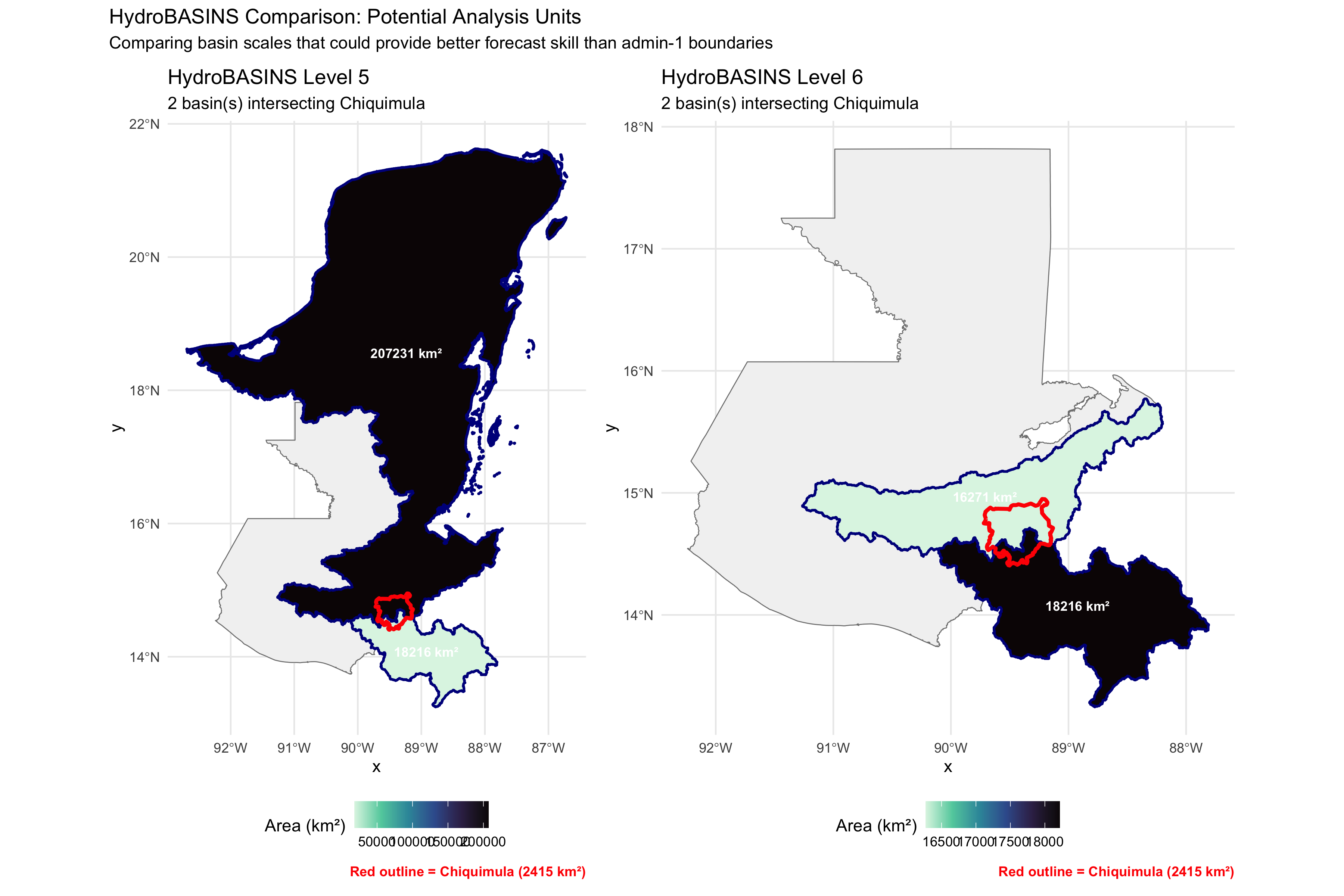
Both SEAS5 and INSIVUMEH may perform poorly at the admin-1 (Chiquimula) scale because seasonal forecasts typically have better skill at larger spatial scales. HydroBASINS provides standardized watershed boundaries at multiple levels that could serve as alternative analysis units.

Load HydroBASINS and Chiquimula boundary

library(tidyverse)
library(sf)
library(cumulus)

# Disable s2 for this section (HydroBASINS has some geometry issues with s2)
sf_use_s2(FALSE)

# Load Guatemala boundaries
sf_gtm_adm0 <- cumulus::download_fieldmaps_sf(iso3 = "GTM", layer = "gtm_adm0")$gtm_adm0
sf_gtm_adm1 <- cumulus::download_fieldmaps_sf(iso3 = "GTM", layer = "gtm_adm1")$gtm_adm1 |>
 janitor::clean_names()
sf_chiquimula <- sf_gtm_adm1 |> filter(adm1_pcode == "GT20")

# Path to HydroBASINS data
hybas_dir <- "../../data/hybas_na_lev01-12_v1c"

# Load levels 5 and 6
sf_hybas_5 <- st_read(file.path(hybas_dir, "hybas_na_lev05_v1c.shp"), quiet = TRUE)
sf_hybas_6 <- st_read(file.path(hybas_dir, "hybas_na_lev06_v1c.shp"), quiet = TRUE)

# Ensure same CRS
sf_chiquimula <- st_transform(sf_chiquimula, st_crs(sf_hybas_5))

# Get bounding box of Chiquimula with buffer for context
chiq_bbox <- st_bbox(sf_chiquimula)
bbox_buffer <- 1  # degrees

# Create bbox polygon for filtering
bbox_poly <- st_as_sfc(st_bbox(c(
  xmin = as.numeric(chiq_bbox["xmin"]) - bbox_buffer,
  xmax = as.numeric(chiq_bbox["xmax"]) + bbox_buffer,
  ymin = as.numeric(chiq_bbox["ymin"]) - bbox_buffer,
  ymax = as.numeric(chiq_bbox["ymax"]) + bbox_buffer
), crs = st_crs(sf_hybas_5)))

# Filter basins to region around Chiquimula using intersection
sf_hybas_5_region <- sf_hybas_5[st_intersects(sf_hybas_5, bbox_poly, sparse = FALSE)[,1], ]
sf_hybas_6_region <- sf_hybas_6[st_intersects(sf_hybas_6, bbox_poly, sparse = FALSE)[,1], ]

# Find basins that intersect Chiquimula
sf_hybas_5_intersect <- sf_hybas_5_region[st_intersects(sf_hybas_5_region, sf_chiquimula, sparse = FALSE)[,1], ]
sf_hybas_6_intersect <- sf_hybas_6_region[st_intersects(sf_hybas_6_region, sf_chiquimula, sparse = FALSE)[,1], ]

cat("Level 5 basins intersecting Chiquimula:", nrow(sf_hybas_5_intersect), "\n")

Level 5 basins intersecting Chiquimula: 2

Load HydroBASINS and Chiquimula boundary

cat("Level 6 basins intersecting Chiquimula:", nrow(sf_hybas_6_intersect), "\n")

Level 6 basins intersecting Chiquimula: 2

Map comparing basin levels 5 and 6 over Chiquimula

library(patchwork)

# Calculate areas for labels
sf_hybas_5_intersect <- sf_hybas_5_intersect |>
  mutate(area_km2 = as.numeric(st_area(geometry)) / 1e6)

sf_hybas_6_intersect <- sf_hybas_6_intersect |>
  mutate(area_km2 = as.numeric(st_area(geometry)) / 1e6)

chiq_area <- as.numeric(st_area(sf_chiquimula)) / 1e6

# Transform admin0 to match CRS
sf_gtm_adm0_t <- st_transform(sf_gtm_adm0, st_crs(sf_hybas_5))

# Create base plot function
create_basin_map <- function(sf_basins, level, sf_admin, sf_country) {

  # Get centroids for labels
  basin_centroids <- st_centroid(sf_basins) |>
    mutate(
      x = st_coordinates(geometry)[,1],
      y = st_coordinates(geometry)[,2]
    )

  ggplot() +
    geom_sf(data = sf_country, fill = "grey95", color = "grey50", linewidth = 0.3) +
    geom_sf(data = sf_basins, aes(fill = area_km2), color = "darkblue", linewidth = 0.8) +
    geom_sf(data = sf_admin, fill = NA, color = "red", linewidth = 1.2) +
    geom_sf_text(
      data = basin_centroids,
      aes(label = paste0(round(area_km2), " km²")),
      size = 3, fontface = "bold", color = "white"
    ) +
    scale_fill_viridis_c(option = "mako", direction = -1, name = "Area (km²)") +
    labs(
      title = paste0("HydroBASINS Level ", level),
      subtitle = paste0(nrow(sf_basins), " basin(s) intersecting Chiquimula"),
      caption = paste0("Red outline = Chiquimula (", round(chiq_area), " km²)")
    ) +
    theme_minimal() +
    theme(
      legend.position = "bottom",
      plot.caption = element_text(color = "red", face = "bold")
    )
}

p_lev5 <- create_basin_map(sf_hybas_5_intersect, 5, sf_chiquimula, sf_gtm_adm0_t)
p_lev6 <- create_basin_map(sf_hybas_6_intersect, 6, sf_chiquimula, sf_gtm_adm0_t)

p_lev5 + p_lev6 +
  plot_annotation(
    title = "HydroBASINS Comparison: Potential Analysis Units",
    subtitle = "Comparing basin scales that could provide better forecast skill than admin-1 boundaries"
  )

Code

# Summary comparison
tibble(
  `Spatial Unit` = c(
    "Chiquimula (Admin-1)",
    paste0("Level 5 (", nrow(sf_hybas_5_intersect), " basin", ifelse(nrow(sf_hybas_5_intersect) > 1, "s", ""), ")"),
    paste0("Level 6 (", nrow(sf_hybas_6_intersect), " basin", ifelse(nrow(sf_hybas_6_intersect) > 1, "s", ""), ")")
  ),
  `Total Area (km²)` = c(
    round(chiq_area),
    round(sum(sf_hybas_5_intersect$area_km2)),
    round(sum(sf_hybas_6_intersect$area_km2))
  ),
  `Mean Basin Area (km²)` = c(
    round(chiq_area),
    round(mean(sf_hybas_5_intersect$area_km2)),
    round(mean(sf_hybas_6_intersect$area_km2))
  ),
  Notes = c(
    "Current analysis unit",
    "Larger basins - may have better forecast skill",
    "Medium basins - balance of skill and resolution"
  )
) |>
  knitr::kable(caption = "Comparison of spatial units for forecast skill assessment")

Comparison of spatial units for forecast skill assessment
Spatial Unit	Total Area (km²)	Mean Basin Area (km²)	Notes
Chiquimula (Admin-1)	2415	2415	Current analysis unit
Level 5 (2 basins)	225446	112723	Larger basins - may have better forecast skill
Level 6 (2 basins)	34487	17243	Medium basins - balance of skill and resolution

A.4.1 Original Interpretation

Level 5 provides larger drainage basins that may better match the spatial resolution at which seasonal forecasts have skill
Level 6 offers a middle ground between admin boundaries and larger regional basins

This avenue was not pursued further after the internal consistency analysis (Chapter 5) revealed that the INSIVUMEH Postrera forecasts lack meaningful signal at any spatial scale.