7  CADC - Framework Skill Comparison

7.1 Overview

This chapter extends the skill assessment beyond Chiquimula (Guatemala) to examine SEAS5 forecast performance across the Central American Dry Corridor, comparing:

  • Guatemala (Chiquimula - GT20)
  • Honduras (El Paraíso + Francisco Morazán - HN07/HN08, area-weighted)
  • El Salvador (Ahuachapán + Santa Ana - SV01/SV12, area-weighted).

We evaluate how skill varies by:

  1. Season: Primera (May-Aug) vs Postrera (Sep-Nov)
  2. Leadtime: LT0-2 for Primera, LT0-3 for Postrera
  3. Baseline period: 2000-2024 (25 years) vs 1990-2024 (35 years) vs 1981-2024 (44 years)

7.2 Data Preparation

Code
PRIMERA_MONTHS <- 5:8
POSTRERA_MONTHS <- 9:11
PRIMERA_ISSUED_MONTHS <- c(3, 4, 5)
POSTRERA_ISSUED_MONTHS <- c(6, 7, 8, 9)

# Toggle AOI sets: comment/uncomment to switch
# 2025 framework (single admin per country)
# SLV_PCODES <- c("SV11")
# 2026 framework (multi-admin weighted)
SLV_PCODES <- c("SV01", "SV12")

AOI_PCODES <- c("HN07", "HN08", SLV_PCODES, "GT20")

# Map pcodes to country labels
pcode_to_country <- function(pcode) {
  case_when(
    pcode == "GT20" ~ "Guatemala",
    pcode %in% c("HN07", "HN08") ~ "Honduras",
    pcode %in% SLV_PCODES ~ "El Salvador"
  )
}

con <- pg_con()

df_weights <- tbl(con, "polygon") |>
  mutate(across(pcode, as.character)) |>
  filter(adm_level == 1, pcode %in% AOI_PCODES) |>
  select(pcode, iso3, name, seas5_n_upsampled_pixels) |>
  collect()

df_seas5_raw <- tbl(con, "seas5") |>
  mutate(across(pcode, as.character)) |>
  filter(adm_level == 1, pcode %in% AOI_PCODES) |>
  collect()

df_era5_raw <- tbl(con, "era5") |>
  mutate(across(pcode, as.character)) |>
  filter(pcode %in% AOI_PCODES) |>
  collect()

DBI::dbDisconnect(con)

# Process to seasonal totals
df_seas5_mm <- df_seas5_raw |>
  mutate(value_mm = days_in_month(valid_date) * mean)

df_seas5_seasonal <- bind_rows(
  seas5_aggregate_forecast(df_seas5_mm, value = "value_mm", valid_months = PRIMERA_MONTHS,
                           by = c("iso3", "pcode", "issued_date")) |> mutate(window = "primera"),
  seas5_aggregate_forecast(df_seas5_mm, value = "value_mm", valid_months = POSTRERA_MONTHS,
                           by = c("iso3", "pcode", "issued_date")) |> mutate(window = "postrera")
) |>
  rename(fcst_mm = value_mm) |>
  mutate(
    year = year(issued_date),
    issued_month = month(issued_date)
  ) |>
  filter(
    (window == "primera" & issued_month %in% PRIMERA_ISSUED_MONTHS) |
    (window == "postrera" & issued_month %in% POSTRERA_ISSUED_MONTHS)
  )

df_era5_monthly <- df_era5_raw |>
  mutate(
    year = year(valid_date),
    month = month(valid_date),
    value_mm = mean * days_in_month(valid_date)
  )
# aggregate temporally
df_era5_seasonal <- bind_rows(
  df_era5_monthly |>
    filter(month %in% PRIMERA_MONTHS) |>
    group_by(pcode, iso3, year) |>
    summarise(obs_mm = sum(value_mm), .groups = "drop") |>
    mutate(window = "primera"),
  df_era5_monthly |>
    filter(month %in% POSTRERA_MONTHS) |>
    group_by(pcode, iso3, year) |>
    summarise(obs_mm = sum(value_mm), .groups = "drop") |>
    mutate(window = "postrera")
)

# Also create country-level ERA5 for yearly RP heatmaps
df_obs_country <- df_era5_seasonal |>
 left_join(df_weights |> select(pcode, seas5_n_upsampled_pixels), by = "pcode") |>
  mutate(
    country_aoi = pcode_to_country(pcode)
  ) |>
  group_by(country_aoi, year, window) |>
  summarise(
    obs_mm = weighted.mean(obs_mm, w = seas5_n_upsampled_pixels),
    .groups = "drop"
  )

# Join and aggregate to country level (weighted mean for Honduras)
df_joined <- df_seas5_seasonal |>
  left_join(
    df_era5_seasonal |> select(pcode, year, window, obs_mm),
    by = c("pcode", "year", "window")
  ) |>
  filter(!is.na(obs_mm)) |>
  left_join(df_weights |> select(pcode, seas5_n_upsampled_pixels), by = "pcode") |>
  mutate(
    country_aoi = pcode_to_country(pcode)
  ) |>
  filter(!is.na(country_aoi)) |>
  group_by(country_aoi, year, window, leadtime, issued_date) |>
  # aggregate geographically via weighted mean
  summarise(
    fcst_mm = weighted.mean(fcst_mm, w = seas5_n_upsampled_pixels),
    obs_mm = weighted.mean(obs_mm, w = seas5_n_upsampled_pixels),
    .groups = "drop"
  )
Code
# =============================================================================
# RP threshold calculation - consistent with other chapters
# Uses proper ranking with interpolation (not simple quantile)
# =============================================================================
calc_rp_threshold <- function(x, rp_target = 4, direction = -1) {
  x <- x[!is.na(x)]
  n <- length(x)
  if (n < 3) return(NA_real_)

  # Use proper ranking with tie handling

# For direction = -1 (drought/low extreme): lowest values get rank 1 (highest RP)
  ranks <- rank(x * -direction, ties.method = "average")
  rp <- (n + 1) / ranks

  # Interpolate to find value at target RP
  approx(rp, x, xout = rp_target, rule = 2)$y
}

# =============================================================================
# Skill metrics calculation using yardstick
# =============================================================================
calc_skill_metrics <- function(df, baseline_start, baseline_end) {
  df_baseline <- df |>
    filter(year >= baseline_start, year <= baseline_end)

  # Calculate observation thresholds per country/window
  obs_thresholds <- df_baseline |>
    group_by(country_aoi, window) |>
    summarise(obs_thresh = calc_rp_threshold(obs_mm, 4, -1), .groups = "drop")

  # Calculate forecast thresholds per country/window/leadtime
  fcst_thresholds <- df_baseline |>
    group_by(country_aoi, window, leadtime) |>
    summarise(fcst_thresh = calc_rp_threshold(fcst_mm, 4, -1), .groups = "drop")

  # Classify and create factors with proper levels for yardstick
  # CRITICAL: drought must be first level (positive class)
  # Using forcats::fct() for stricter validation (errors if values don't match levels)
  drought_levels <- c("drought", "no_drought")

df_classified <- df_baseline |>
    left_join(obs_thresholds, by = c("country_aoi", "window")) |>
    left_join(fcst_thresholds, by = c("country_aoi", "window", "leadtime")) |>
    mutate(
      # Truth: was it actually a drought?
      truth = fct(
        if_else(obs_mm <= obs_thresh, "drought", "no_drought"),
        levels = drought_levels
      ),
      # Estimate: did we predict drought?
      estimate = fct(
        if_else(fcst_mm <= fcst_thresh, "drought", "no_drought"),
        levels = drought_levels
      )
    ) |>
    filter(!is.na(truth), !is.na(estimate))

  # Calculate metrics using yardstick
  df_classified |>
    group_by(country_aoi, window, leadtime) |>
    summarise(
      n_years = n_distinct(year),
      n_drought = sum(truth == "drought"),

      # Spearman correlation (continuous)
      spearman = cor(fcst_mm, obs_mm, method = "spearman", use = "complete.obs"),

      # ROC-AUC: lower forecast = predict drought, so negate fcst_mm
      # yardstick returns NA (with warning) if only one class present
      roc_auc = roc_auc_vec(truth, -fcst_mm, event_level = "first"),

      # F1 using yardstick (event_level = "first" means drought is positive class)
      f1 = f_meas_vec(truth, estimate, event_level = "first"),
      precision = precision_vec(truth, estimate, event_level = "first"),
      recall = recall_vec(truth, estimate, event_level = "first"),

      .groups = "drop"
    ) |>
    select(country_aoi, window, leadtime, n_years, n_drought, spearman, roc_auc, f1)
}

df_skill_2000 <- calc_skill_metrics(df_joined, 2000, 2024) |> mutate(baseline = "2000-2024")
df_skill_1991 <- calc_skill_metrics(df_joined, 1991, 2024) |> mutate(baseline = "1991-2024")
df_skill_1990 <- calc_skill_metrics(df_joined, 1990, 2024) |> mutate(baseline = "1990-2024")
df_skill_1981 <- calc_skill_metrics(df_joined, 1981, 2024) |> mutate(baseline = "1981-2024")

df_skill_all <- bind_rows(df_skill_2000, df_skill_1991, df_skill_1990, df_skill_1981) |>
  mutate(
    baseline = factor(baseline, levels = c("2000-2024", "1991-2024", "1990-2024", "1981-2024")),
    window = factor(window, levels = c("primera", "postrera")),
    country_aoi = factor(country_aoi, levels = c("Guatemala", "Honduras", "El Salvador"))
  )

7.3 Primera: Consistently Skillful

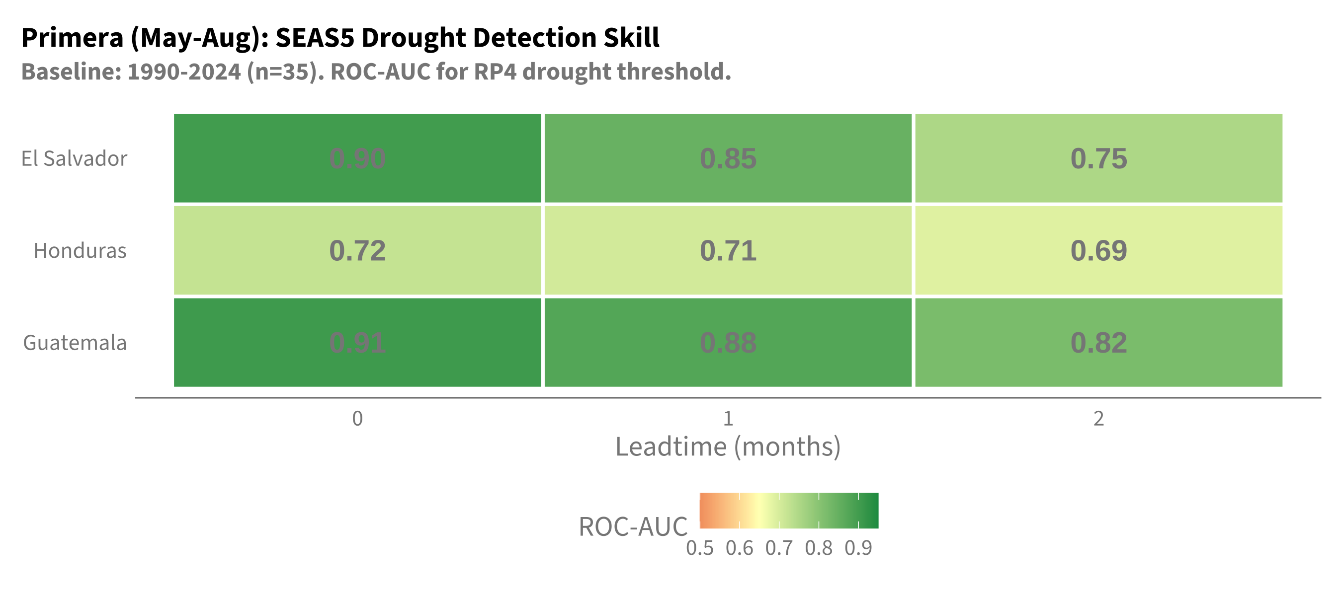
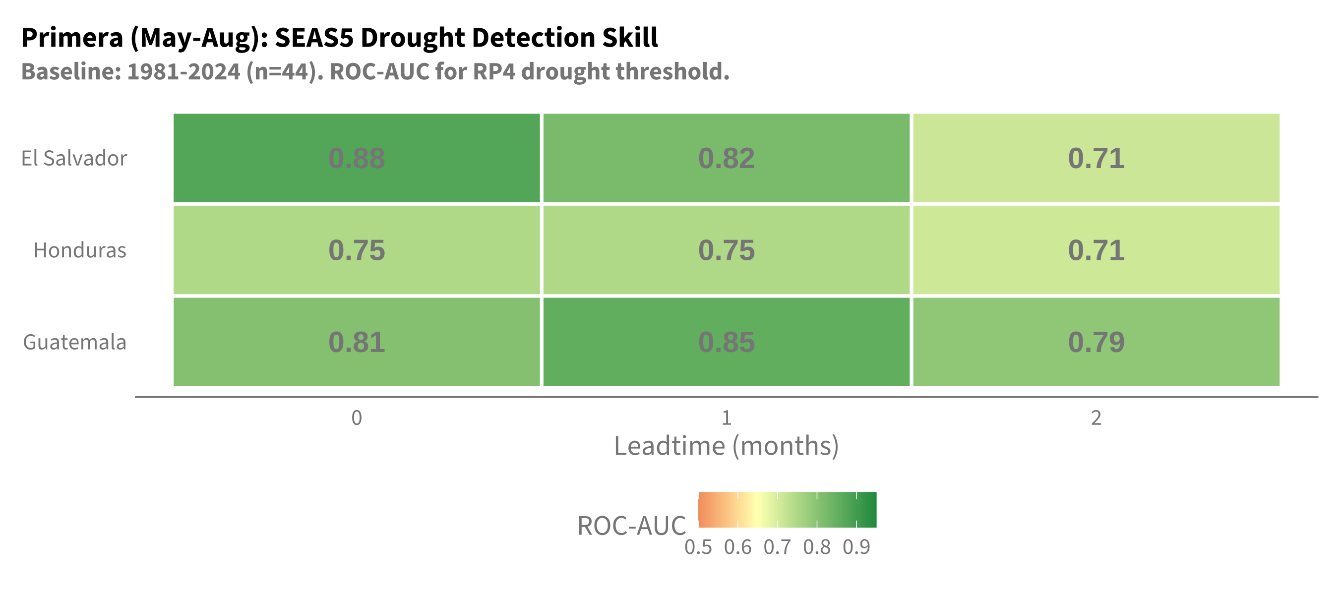
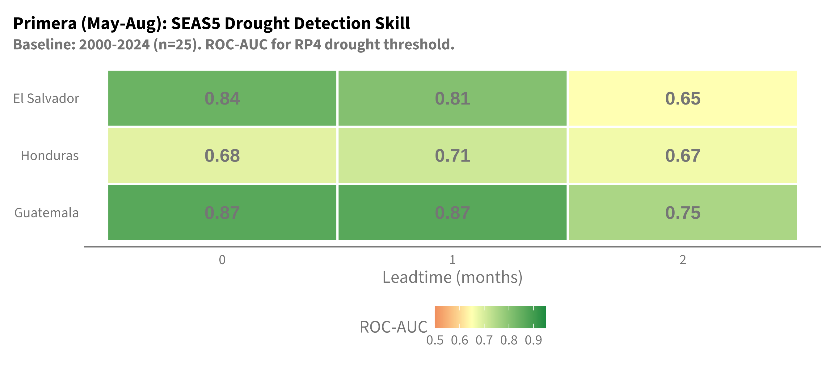
Primera forecasts show acceptable skill across all three countries, with ROC-AUC values consistently above 0.65 and reaching 0.85+ for Guatemala at shorter leadtimes.

Code
df_skill_all |>
  filter(window == "primera", leadtime %in% c(0, 1, 2), baseline == "2000-2024") |>
  ggplot(aes(x = factor(leadtime), y = country_aoi, fill = roc_auc)) +
  geom_tile(color = "white", linewidth = 0.8) +
  geom_text(aes(label = sprintf("%.2f", roc_auc)), size = 5, fontface = "bold") +
  scale_fill_gradient2(
    low = "#D73027", mid = "#FFFFBF", high = "#1A9850",
    midpoint = 0.65, limits = c(0.5, 0.95), name = "ROC-AUC",
    oob = scales::squish
  ) +
  labs(
    title = "Primera (May-Aug): SEAS5 Drought Detection Skill",
    subtitle = "Baseline: 2000-2024 (n=25). ROC-AUC for RP4 drought threshold.",
    x = "Leadtime (months)", y = NULL
  ) +
  theme(
    panel.grid = element_blank(),
    plot.title = element_text(size = 14, face = "bold")
  )

Code
df_skill_all |>
  filter(window == "primera", leadtime %in% c(0, 1, 2), baseline == "1990-2024") |>
  ggplot(aes(x = factor(leadtime), y = country_aoi, fill = roc_auc)) +
  geom_tile(color = "white", linewidth = 0.8) +
  geom_text(aes(label = sprintf("%.2f", roc_auc)), size = 5, fontface = "bold") +
  scale_fill_gradient2(
    low = "#D73027", mid = "#FFFFBF", high = "#1A9850",
    midpoint = 0.65, limits = c(0.5, 0.95), name = "ROC-AUC",
    oob = scales::squish
  ) +
  labs(
    title = "Primera (May-Aug): SEAS5 Drought Detection Skill",
    subtitle = "Baseline: 1990-2024 (n=35). ROC-AUC for RP4 drought threshold.",
    x = "Leadtime (months)", y = NULL
  ) +
  theme(
    panel.grid = element_blank(),
    plot.title = element_text(size = 14, face = "bold")
  )

Code
df_skill_all |>
  filter(window == "primera", leadtime %in% c(0, 1, 2), baseline == "1981-2024") |>
  ggplot(aes(x = factor(leadtime), y = country_aoi, fill = roc_auc)) +
  geom_tile(color = "white", linewidth = 0.8) +
  geom_text(aes(label = sprintf("%.2f", roc_auc)), size = 5, fontface = "bold") +
  scale_fill_gradient2(
    low = "#D73027", mid = "#FFFFBF", high = "#1A9850",
    midpoint = 0.65, limits = c(0.5, 0.95), name = "ROC-AUC",
    oob = scales::squish
  ) +
  labs(
    title = "Primera (May-Aug): SEAS5 Drought Detection Skill",
    subtitle = "Baseline: 1981-2024 (n=44). ROC-AUC for RP4 drought threshold.",
    x = "Leadtime (months)", y = NULL
  ) +
  theme(
    panel.grid = element_blank(),
    plot.title = element_text(size = 14, face = "bold")
  )

Key finding: Primera skill is robust across AOIs and baseline periods. The choice of baseline has minimal impact on Primera performance.

7.4 Postrera: Baseline Period Matters

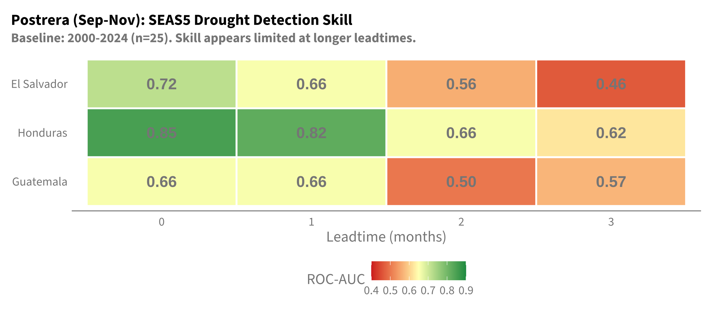
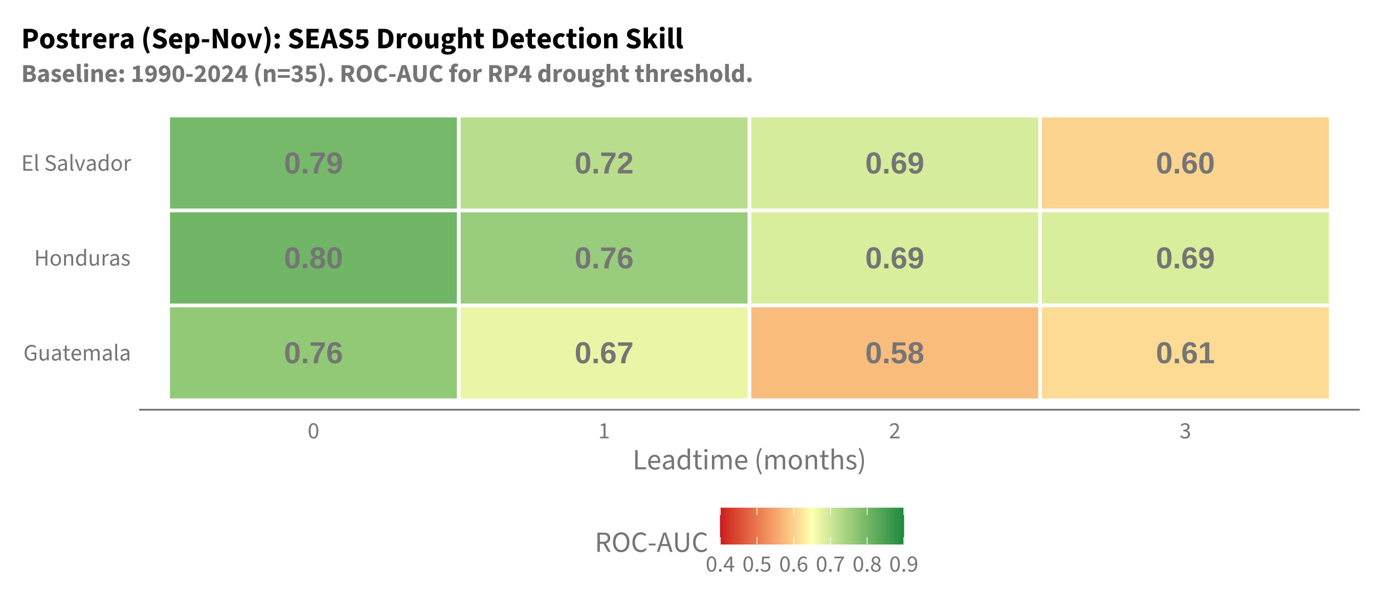
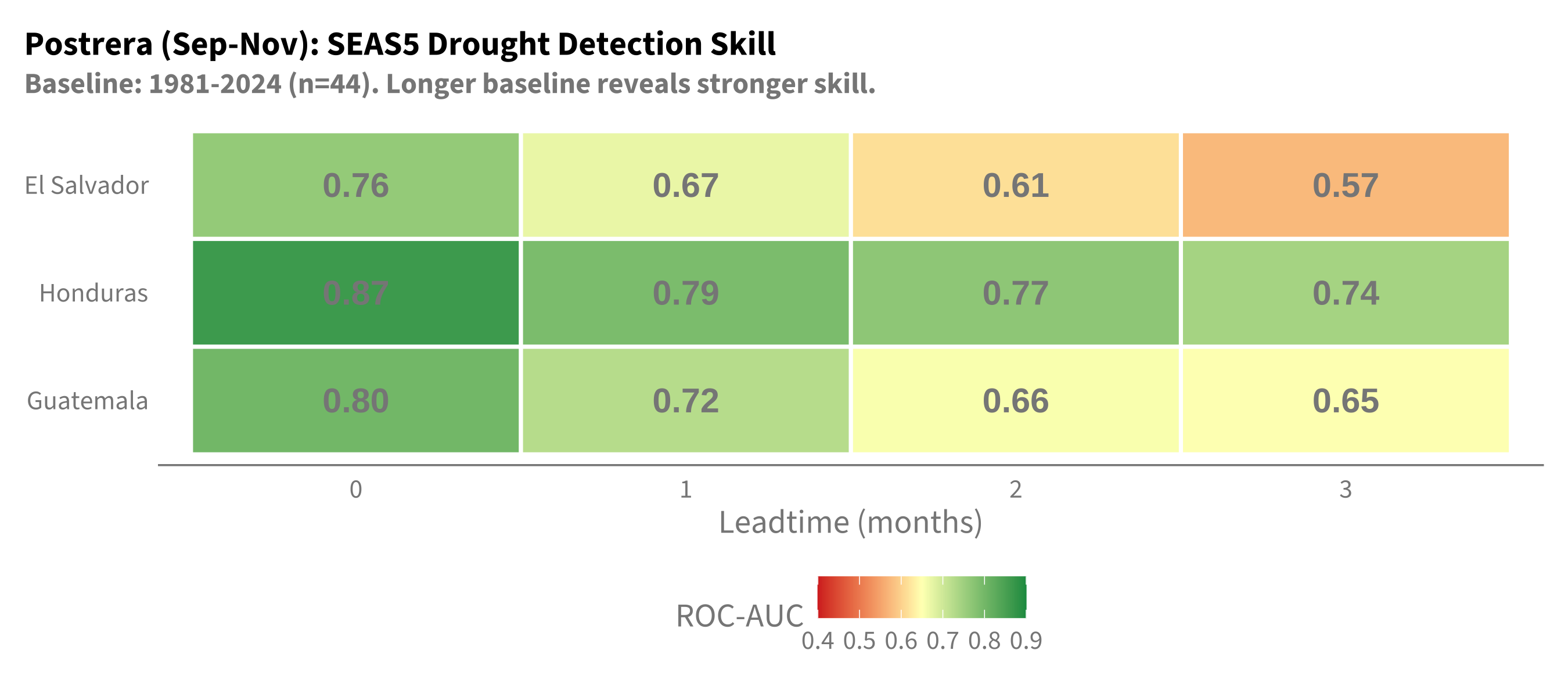
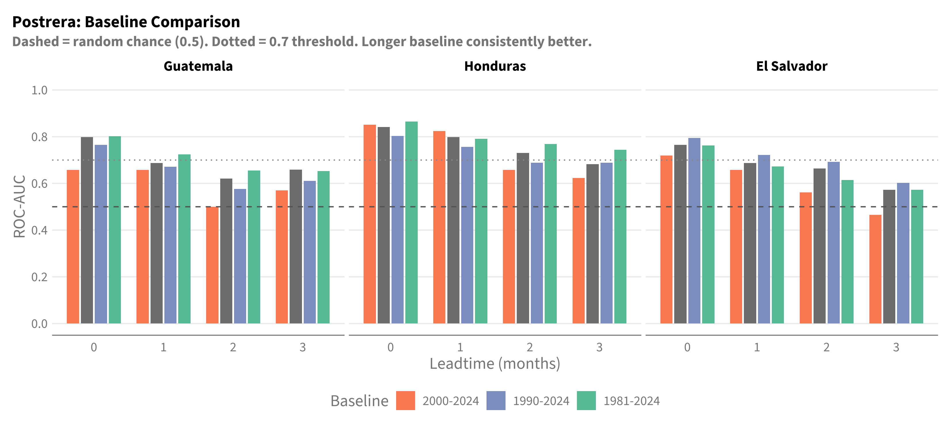
Postrera presents a more complex picture. The 2000-2024 baseline suggests limited skill, but extending to 1981-2024 reveals substantially better performance.

Code
df_skill_all |>
  filter(window == "postrera", leadtime %in% c(0, 1, 2, 3), baseline == "2000-2024") |>
  ggplot(aes(x = factor(leadtime), y = country_aoi, fill = roc_auc)) +
  geom_tile(color = "white", linewidth = 0.8) +
  geom_text(aes(label = sprintf("%.2f", roc_auc)), size = 5, fontface = "bold") +
  scale_fill_gradient2(
    low = "#D73027", mid = "#FFFFBF", high = "#1A9850",
    midpoint = 0.65, limits = c(0.4, 0.9), name = "ROC-AUC",
    oob = scales::squish
  ) +
  labs(
    title = "Postrera (Sep-Nov): SEAS5 Drought Detection Skill",
    subtitle = "Baseline: 2000-2024 (n=25). Skill appears limited at longer leadtimes.",
    x = "Leadtime (months)", y = NULL
  ) +
  theme(
    panel.grid = element_blank(),
    plot.title = element_text(size = 14, face = "bold")
  )

Code
df_skill_all |>
  filter(window == "postrera", leadtime %in% c(0, 1, 2, 3), baseline == "1990-2024") |>
  ggplot(aes(x = factor(leadtime), y = country_aoi, fill = roc_auc)) +
  geom_tile(color = "white", linewidth = 0.8) +
  geom_text(aes(label = sprintf("%.2f", roc_auc)), size = 5, fontface = "bold") +
  scale_fill_gradient2(
    low = "#D73027", mid = "#FFFFBF", high = "#1A9850",
    midpoint = 0.65, limits = c(0.4, 0.9), name = "ROC-AUC",
    oob = scales::squish
  ) +
  labs(
    title = "Postrera (Sep-Nov): SEAS5 Drought Detection Skill",
    subtitle = "Baseline: 1990-2024 (n=35). ROC-AUC for RP4 drought threshold.",
    x = "Leadtime (months)", y = NULL
  ) +
  theme(
    panel.grid = element_blank(),
    plot.title = element_text(size = 14, face = "bold")
  )

Code
df_skill_all |>
  filter(window == "postrera", leadtime %in% c(0, 1, 2, 3), baseline == "1981-2024") |>
  ggplot(aes(x = factor(leadtime), y = country_aoi, fill = roc_auc)) +
  geom_tile(color = "white", linewidth = 0.8) +
  geom_text(aes(label = sprintf("%.2f", roc_auc)), size = 5, fontface = "bold") +
  scale_fill_gradient2(
    low = "#D73027", mid = "#FFFFBF", high = "#1A9850",
    midpoint = 0.65, limits = c(0.4, 0.9), name = "ROC-AUC",
    oob = scales::squish
  ) +
  labs(
    title = "Postrera (Sep-Nov): SEAS5 Drought Detection Skill",
    subtitle = "Baseline: 1981-2024 (n=44). Longer baseline reveals stronger skill.",
    x = "Leadtime (months)", y = NULL
  ) +
  theme(
    panel.grid = element_blank(),
    plot.title = element_text(size = 14, face = "bold")
  )

Code
df_skill_all |>
  filter(window == "postrera", leadtime %in% c(0, 1, 2, 3)) |>
  ggplot(aes(x = factor(leadtime), y = roc_auc, fill = baseline)) +
  geom_col(position = position_dodge(width = 0.8), width = 0.7) +
  geom_hline(yintercept = 0.5, linetype = "dashed", color = "grey40") +
  geom_hline(yintercept = 0.7, linetype = "dotted", color = "grey60") +
  facet_wrap(~country_aoi) +
  scale_fill_manual(values = c("2000-2024" = "#fc8d62", "1990-2024" = "#8da0cb", "1981-2024" = "#66c2a5")) +
  scale_y_continuous(limits = c(0, 1), breaks = seq(0, 1, 0.2)) +
  labs(
    title = "Postrera: Baseline Comparison",
    subtitle = "Dashed = random chance (0.5). Dotted = 0.7 threshold. Longer baseline consistently better.",
    x = "Leadtime (months)", y = "ROC-AUC", fill = "Baseline"
  ) +
  theme(
    legend.position = "bottom",
    strip.text = element_text(size = 12, face = "bold"),
    plot.title = element_text(size = 14, face = "bold")
  )

7.4.1 Skill Improvement Table

Code
df_skill_all |>
  filter(window == "postrera", leadtime %in% c(0, 1, 2, 3)) |>
  select(country_aoi, baseline, leadtime, roc_auc) |>
  pivot_wider(names_from = baseline, values_from = roc_auc) |>
  mutate(
    diff_1990 = `1990-2024` - `2000-2024`,
    diff_1981 = `1981-2024` - `2000-2024`
  ) |>
  arrange(country_aoi, leadtime) |>
  gt() |>
  fmt_number(columns = c(`2000-2024`, `1990-2024`, `1981-2024`, diff_1990, diff_1981), decimals = 2) |>
  cols_label(
    country_aoi = "Country",
    leadtime = "LT",
    `2000-2024` = "2000-2024",
    `1990-2024` = "1990-2024",
    `1981-2024` = "1981-2024",
    diff_1990 = "Δ 1990",
    diff_1981 = "Δ 1981"
  ) |>
  tab_header(
    title = "Postrera ROC-AUC: Baseline Comparison",
    subtitle = "Skill improvement from extending baseline (relative to 2000-2024)"
  ) |>
  tab_style(
    style = cell_fill(color = "#d4edda"),
    locations = cells_body(
      columns = c(diff_1990, diff_1981),
      rows = diff_1981 > 0.1
    )
  )
Postrera ROC-AUC: Baseline Comparison
Skill improvement from extending baseline (relative to 2000-2024)
Country LT 2000-2024 1991-2024 1990-2024 1981-2024 Δ 1990 Δ 1981
Guatemala 0 0.66 0.7980769 0.76 0.80 0.11 0.14
Guatemala 1 0.66 0.6875000 0.67 0.72 0.01 0.07
Guatemala 2 0.50 0.6201923 0.58 0.66 0.08 0.16
Guatemala 3 0.57 0.6586538 0.61 0.65 0.04 0.08
Honduras 0 0.85 0.8413462 0.80 0.87 −0.05 0.01
Honduras 1 0.82 0.7980769 0.76 0.79 −0.07 −0.03
Honduras 2 0.66 0.7307692 0.69 0.77 0.03 0.11
Honduras 3 0.62 0.6826923 0.69 0.74 0.07 0.12
El Salvador 0 0.72 0.7644231 0.79 0.76 0.08 0.04
El Salvador 1 0.66 0.6875000 0.72 0.67 0.06 0.01
El Salvador 2 0.56 0.6634615 0.69 0.61 0.13 0.05
El Salvador 3 0.46 0.5721154 0.60 0.57 0.14 0.11

7.4.2 F1 Score by Baseline

Code
df_skill_all |>
  filter(window == "postrera", leadtime %in% c(0, 1, 2, 3), baseline == "1981-2024") |>
  ggplot(aes(x = factor(leadtime), y = country_aoi, fill = f1)) +
  geom_tile(color = "white", linewidth = 0.8) +
  geom_text(aes(label = sprintf("%.2f", f1)), size = 5, fontface = "bold") +
  scale_fill_gradient2(
    low = "#D73027", mid = "#FFFFBF", high = "#1A9850",
    midpoint = 0.4, limits = c(0, 0.8), name = "F1 Score",
    oob = scales::squish, na.value = "grey80"
  ) +
  labs(
    title = "Postrera (Sep-Nov): F1 Score for Drought Classification",
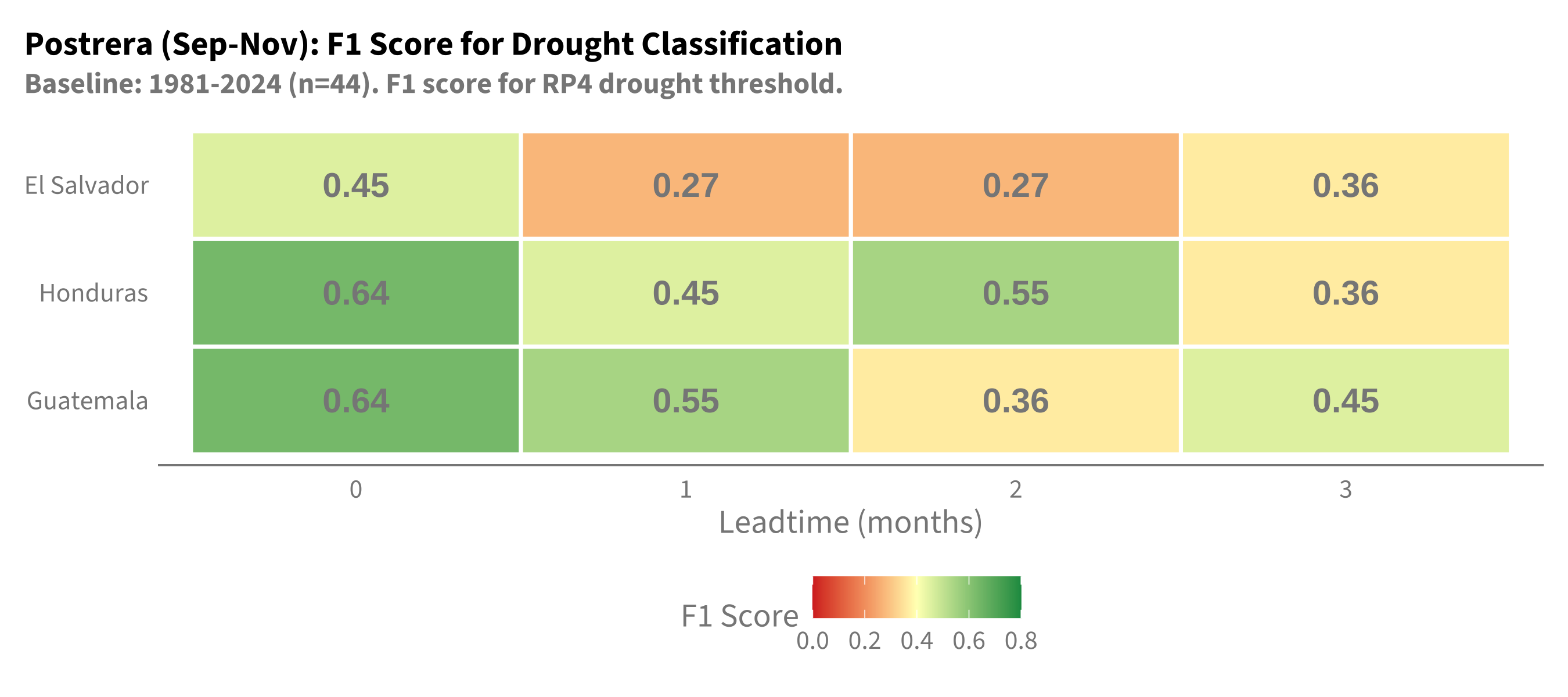
    subtitle = "Baseline: 1981-2024 (n=44). F1 score for RP4 drought threshold.",
    x = "Leadtime (months)", y = NULL
  ) +
  theme(
    panel.grid = element_blank(),
    plot.title = element_text(size = 14, face = "bold")
  )

Code
df_skill_all |>
  filter(window == "postrera", leadtime %in% c(0, 1, 2, 3), baseline == "1991-2024") |>
  ggplot(aes(x = factor(leadtime), y = country_aoi, fill = f1)) +
  geom_tile(color = "white", linewidth = 0.8) +
  geom_text(aes(label = sprintf("%.2f", f1)), size = 5, fontface = "bold") +
  scale_fill_gradient2(
    low = "#D73027", mid = "#FFFFBF", high = "#1A9850",
    midpoint = 0.4, limits = c(0, 0.8), name = "F1 Score",
    oob = scales::squish, na.value = "grey80"
  ) +
  labs(
    title = "Postrera (Sep-Nov): F1 Score for Drought Classification",
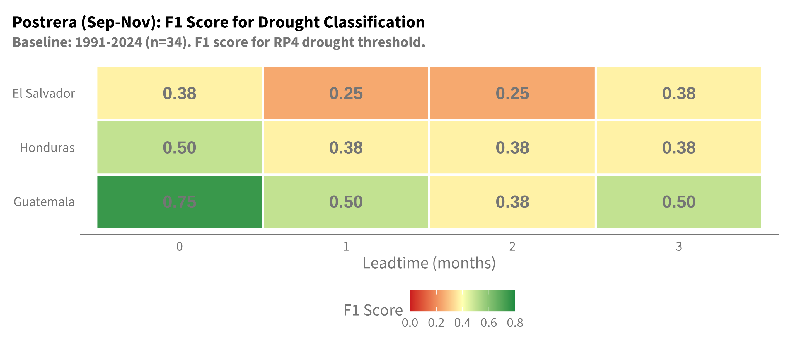
    subtitle = "Baseline: 1991-2024 (n=34). F1 score for RP4 drought threshold.",
    x = "Leadtime (months)", y = NULL
  ) +
  theme(
    panel.grid = element_blank(),
    plot.title = element_text(size = 14, face = "bold")
  )

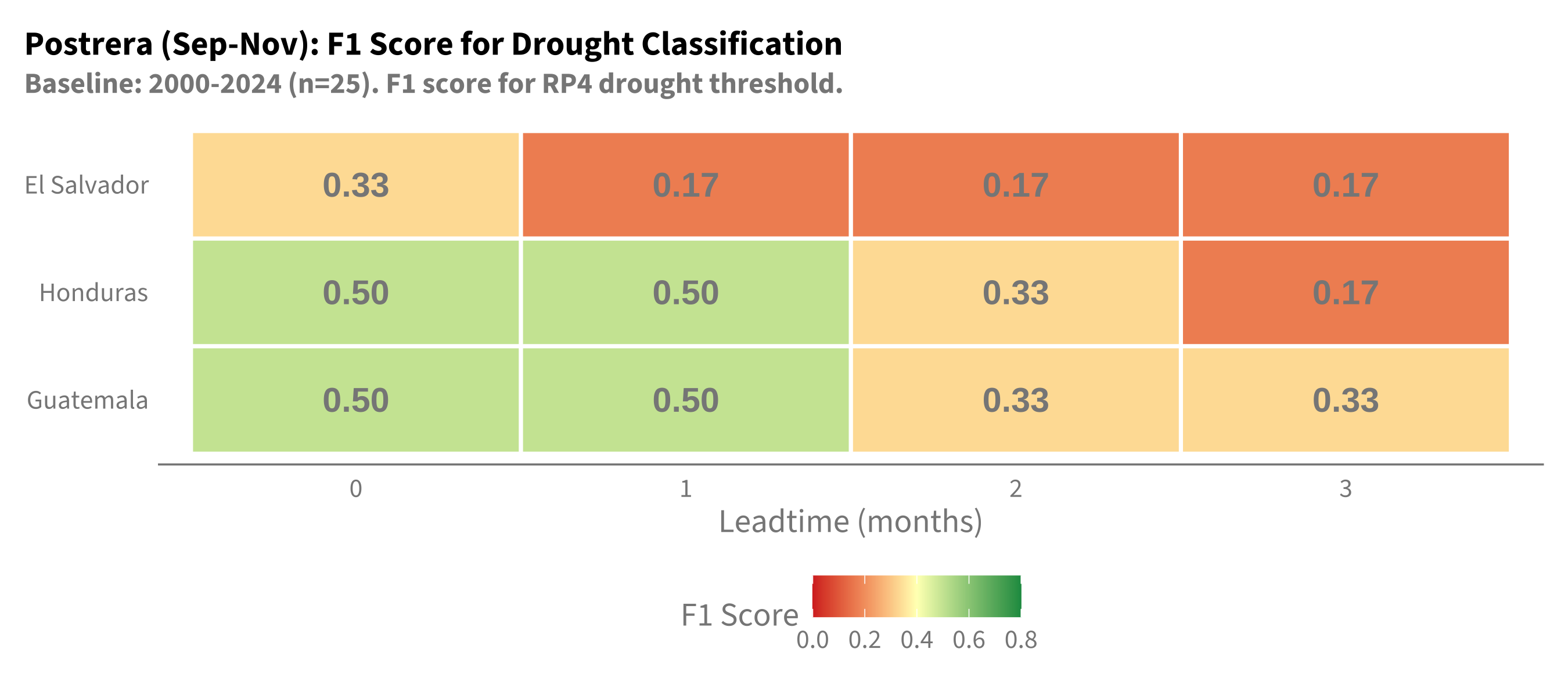
Code
df_skill_all |>
  filter(window == "postrera", leadtime %in% c(0, 1, 2, 3), baseline == "2000-2024") |>
  ggplot(aes(x = factor(leadtime), y = country_aoi, fill = f1)) +
  geom_tile(color = "white", linewidth = 0.8) +
  geom_text(aes(label = sprintf("%.2f", f1)), size = 5, fontface = "bold") +
  scale_fill_gradient2(
    low = "#D73027", mid = "#FFFFBF", high = "#1A9850",
    midpoint = 0.4, limits = c(0, 0.8), name = "F1 Score",
    oob = scales::squish, na.value = "grey80"
  ) +
  labs(
    title = "Postrera (Sep-Nov): F1 Score for Drought Classification",
    subtitle = "Baseline: 2000-2024 (n=25). F1 score for RP4 drought threshold.",
    x = "Leadtime (months)", y = NULL
  ) +
  theme(
    panel.grid = element_blank(),
    plot.title = element_text(size = 14, face = "bold")
  )

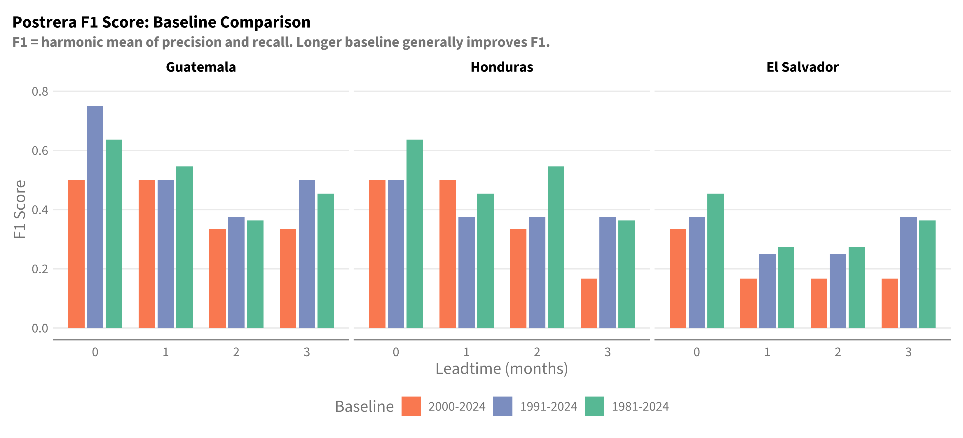
Code
df_skill_all |>
  filter(window == "postrera", leadtime %in% c(0, 1, 2, 3),
         baseline %in% c("1981-2024", "1991-2024", "2000-2024")) |>
  mutate(baseline = factor(baseline, levels = c("2000-2024", "1991-2024", "1981-2024"))) |>
  ggplot(aes(x = factor(leadtime), y = f1, fill = baseline)) +
  geom_col(position = position_dodge(width = 0.8), width = 0.7) +
  facet_wrap(~country_aoi) +
  scale_fill_manual(values = c("2000-2024" = "#fc8d62", "1991-2024" = "#8da0cb", "1981-2024" = "#66c2a5")) +
  scale_y_continuous(limits = c(0, 0.8), breaks = seq(0, 0.8, 0.2)) +
  labs(
    title = "Postrera F1 Score: Baseline Comparison",
    subtitle = "F1 = harmonic mean of precision and recall. Longer baseline generally improves F1.",
    x = "Leadtime (months)", y = "F1 Score", fill = "Baseline"
  ) +
  theme(
    legend.position = "bottom",
    strip.text = element_text(size = 12, face = "bold"),
    plot.title = element_text(size = 14, face = "bold")
  )

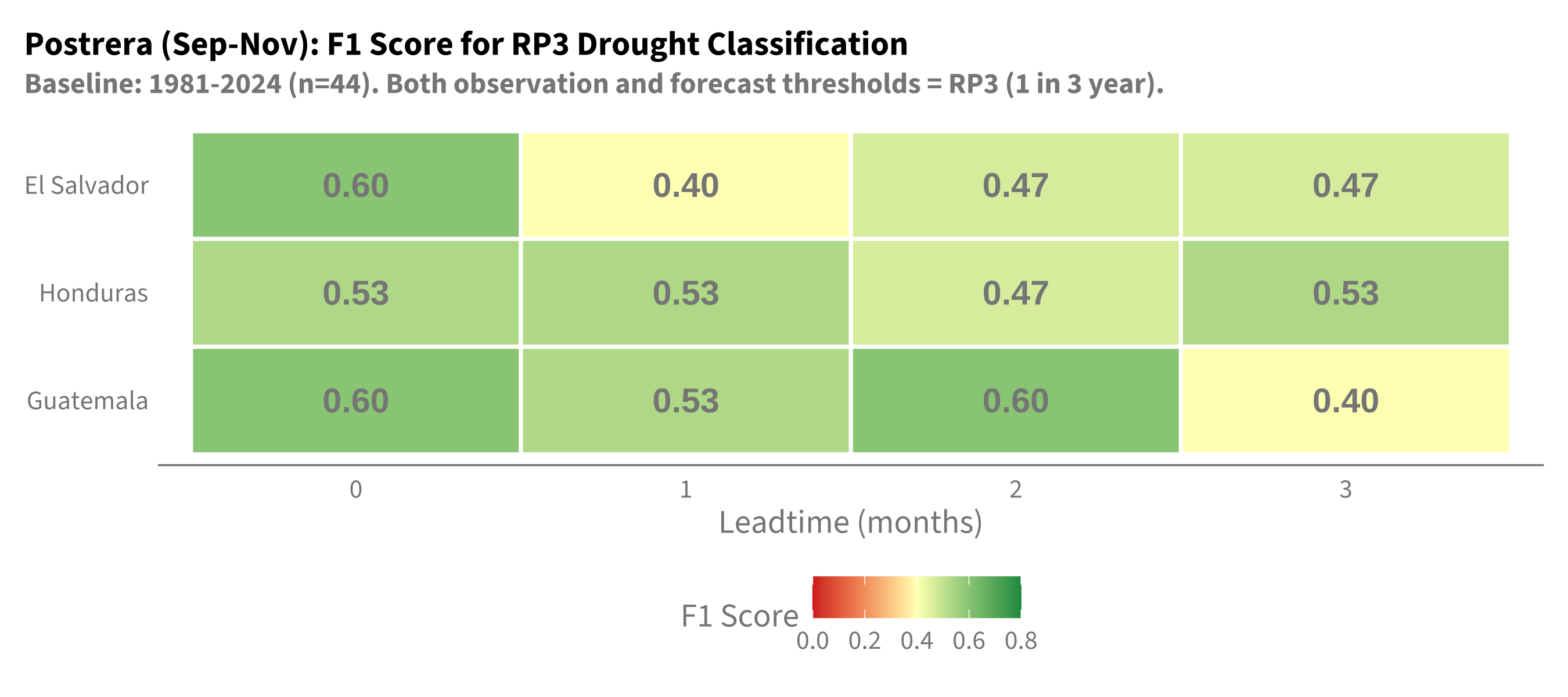
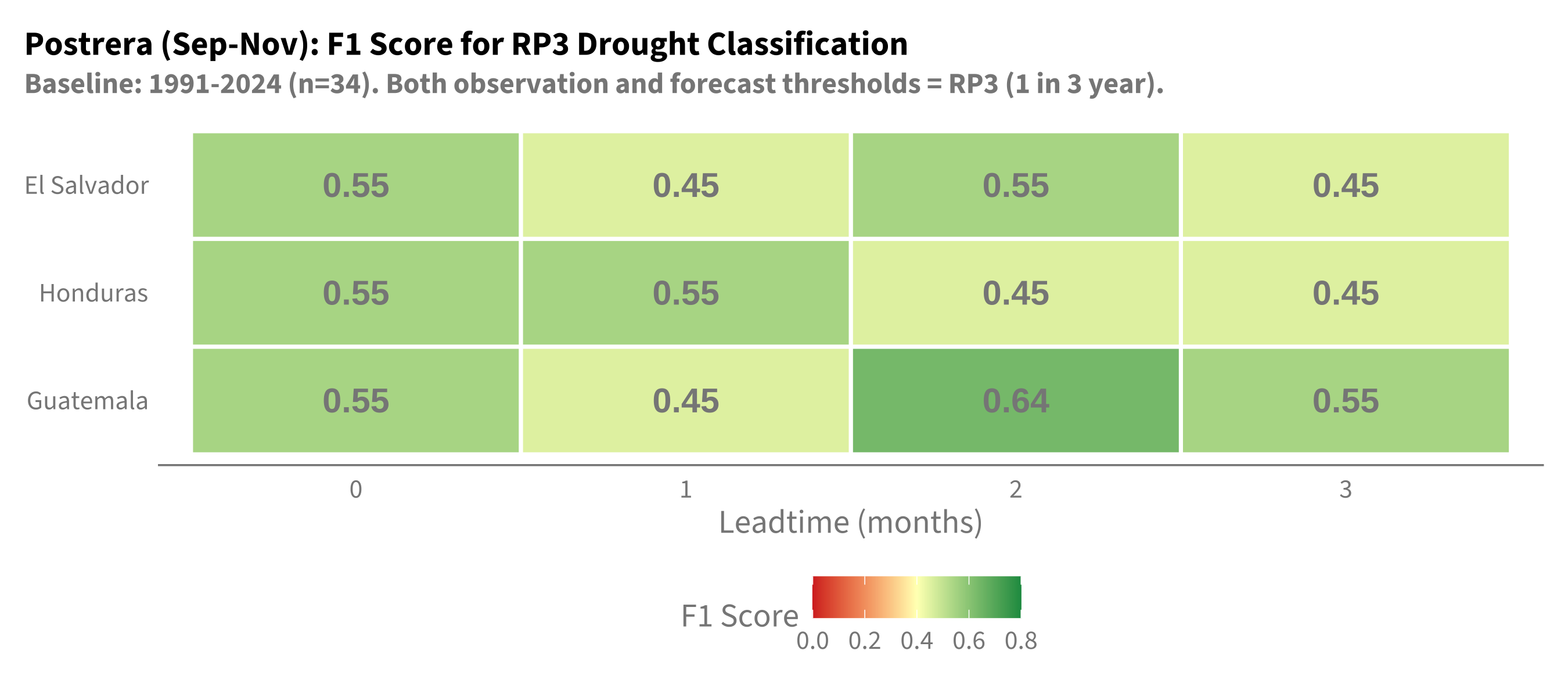
7.4.3 F1 Score with RP3 Threshold (1 in 3 Year Event)

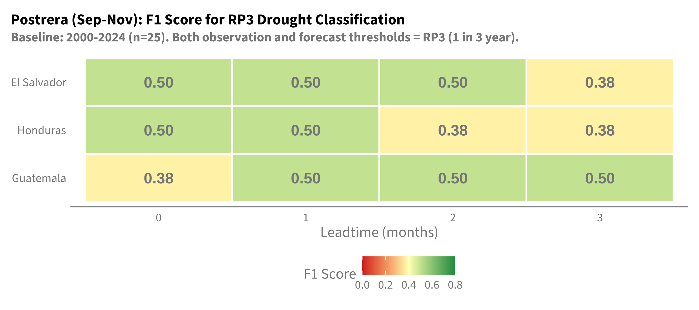
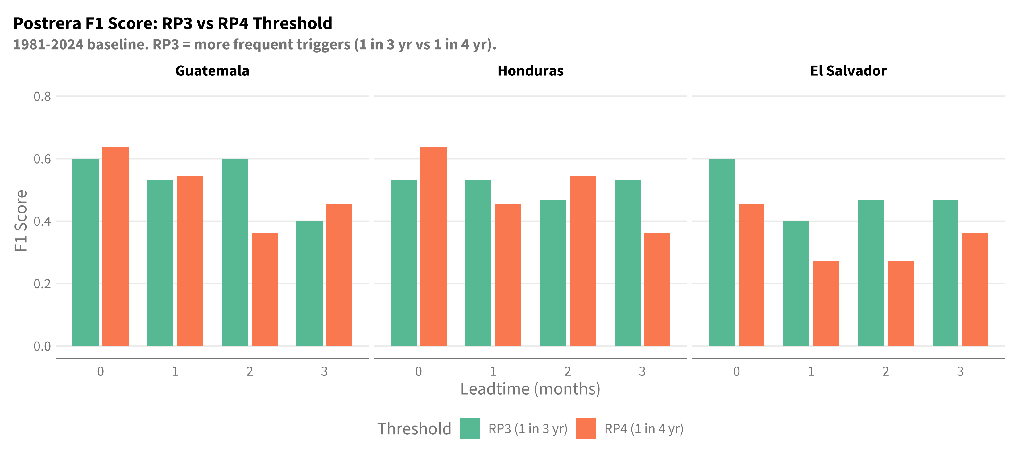
The previous F1 scores use RP4 (1 in 4 year) as the drought definition. Here we examine F1 when both the observation and forecast thresholds are set to RP3 (1 in 3 year event) - a more frequent trigger scenario.

Code
# Calculate skill metrics with RP3 thresholds (both obs and forecast)
calc_skill_metrics_rp3 <- function(df, baseline_start, baseline_end) {
  df_baseline <- df |>
    filter(year >= baseline_start, year <= baseline_end)

  # Calculate observation thresholds at RP3 (more frequent events)
  obs_thresholds <- df_baseline |>
    group_by(country_aoi, window) |>
    summarise(obs_thresh = calc_rp_threshold(obs_mm, 3, -1), .groups = "drop")

  # Calculate forecast thresholds at RP3 (same as obs)
  fcst_thresholds <- df_baseline |>
    group_by(country_aoi, window, leadtime) |>
    summarise(fcst_thresh = calc_rp_threshold(fcst_mm, 3, -1), .groups = "drop")

  drought_levels <- c("drought", "no_drought")

  df_baseline |>
    left_join(obs_thresholds, by = c("country_aoi", "window")) |>
    left_join(fcst_thresholds, by = c("country_aoi", "window", "leadtime")) |>
    mutate(
      truth = fct(
        if_else(obs_mm <= obs_thresh, "drought", "no_drought"),
        levels = drought_levels
      ),
      estimate = fct(
        if_else(fcst_mm <= fcst_thresh, "drought", "no_drought"),
        levels = drought_levels
      )
    ) |>
    filter(!is.na(truth), !is.na(estimate)) |>
    group_by(country_aoi, window, leadtime) |>
    summarise(
      n_years = n_distinct(year),
      n_drought = sum(truth == "drought"),
      spearman = cor(fcst_mm, obs_mm, method = "spearman", use = "complete.obs"),
      roc_auc = roc_auc_vec(truth, -fcst_mm, event_level = "first"),
      f1 = f_meas_vec(truth, estimate, event_level = "first"),
      precision = precision_vec(truth, estimate, event_level = "first"),
      recall = recall_vec(truth, estimate, event_level = "first"),
      .groups = "drop"
    ) |>
    select(country_aoi, window, leadtime, n_years, n_drought, spearman, roc_auc, f1)
}

df_skill_rp3_1981 <- calc_skill_metrics_rp3(df_joined, 1981, 2024) |> mutate(baseline = "1981-2024")
df_skill_rp3_1991 <- calc_skill_metrics_rp3(df_joined, 1991, 2024) |> mutate(baseline = "1991-2024")
df_skill_rp3_2000 <- calc_skill_metrics_rp3(df_joined, 2000, 2024) |> mutate(baseline = "2000-2024")

df_skill_rp3_all <- bind_rows(df_skill_rp3_1981, df_skill_rp3_1991, df_skill_rp3_2000) |>
  mutate(
    baseline = factor(baseline, levels = c("2000-2024", "1991-2024", "1981-2024")),
    window = factor(window, levels = c("primera", "postrera")),
    country_aoi = factor(country_aoi, levels = c("Guatemala", "Honduras", "El Salvador"))
  )
Code
df_skill_rp3_all |>
  filter(window == "postrera", leadtime %in% c(0, 1, 2, 3), baseline == "1981-2024") |>
  ggplot(aes(x = factor(leadtime), y = country_aoi, fill = f1)) +
  geom_tile(color = "white", linewidth = 0.8) +
  geom_text(aes(label = sprintf("%.2f", f1)), size = 5, fontface = "bold") +
  scale_fill_gradient2(
    low = "#D73027", mid = "#FFFFBF", high = "#1A9850",
    midpoint = 0.4, limits = c(0, 0.8), name = "F1 Score",
    oob = scales::squish, na.value = "grey80"
  ) +
  labs(
    title = "Postrera (Sep-Nov): F1 Score for RP3 Drought Classification",
    subtitle = "Baseline: 1981-2024 (n=44). Both observation and forecast thresholds = RP3 (1 in 3 year).",
    x = "Leadtime (months)", y = NULL
  ) +
  theme(
    panel.grid = element_blank(),
    plot.title = element_text(size = 14, face = "bold")
  )

Code
df_skill_rp3_all |>
  filter(window == "postrera", leadtime %in% c(0, 1, 2, 3), baseline == "1991-2024") |>
  ggplot(aes(x = factor(leadtime), y = country_aoi, fill = f1)) +
  geom_tile(color = "white", linewidth = 0.8) +
  geom_text(aes(label = sprintf("%.2f", f1)), size = 5, fontface = "bold") +
  scale_fill_gradient2(
    low = "#D73027", mid = "#FFFFBF", high = "#1A9850",
    midpoint = 0.4, limits = c(0, 0.8), name = "F1 Score",
    oob = scales::squish, na.value = "grey80"
  ) +
  labs(
    title = "Postrera (Sep-Nov): F1 Score for RP3 Drought Classification",
    subtitle = "Baseline: 1991-2024 (n=34). Both observation and forecast thresholds = RP3 (1 in 3 year).",
    x = "Leadtime (months)", y = NULL
  ) +
  theme(
    panel.grid = element_blank(),
    plot.title = element_text(size = 14, face = "bold")
  )

Code
df_skill_rp3_all |>
  filter(window == "postrera", leadtime %in% c(0, 1, 2, 3), baseline == "2000-2024") |>
  ggplot(aes(x = factor(leadtime), y = country_aoi, fill = f1)) +
  geom_tile(color = "white", linewidth = 0.8) +
  geom_text(aes(label = sprintf("%.2f", f1)), size = 5, fontface = "bold") +
  scale_fill_gradient2(
    low = "#D73027", mid = "#FFFFBF", high = "#1A9850",
    midpoint = 0.4, limits = c(0, 0.8), name = "F1 Score",
    oob = scales::squish, na.value = "grey80"
  ) +
  labs(
    title = "Postrera (Sep-Nov): F1 Score for RP3 Drought Classification",
    subtitle = "Baseline: 2000-2024 (n=25). Both observation and forecast thresholds = RP3 (1 in 3 year).",
    x = "Leadtime (months)", y = NULL
  ) +
  theme(
    panel.grid = element_blank(),
    plot.title = element_text(size = 14, face = "bold")
  )

Code
# Compare RP3 vs RP4 F1 scores
df_comparison <- bind_rows(
  df_skill_all |>
    filter(window == "postrera", baseline == "1981-2024") |>
    mutate(obs_threshold = "RP4 (1 in 4 yr)"),
  df_skill_rp3_all |>
    filter(window == "postrera", baseline == "1981-2024") |>
    mutate(obs_threshold = "RP3 (1 in 3 yr)")
)

df_comparison |>
  filter(leadtime %in% c(0, 1, 2, 3)) |>
  ggplot(aes(x = factor(leadtime), y = f1, fill = obs_threshold)) +
  geom_col(position = position_dodge(width = 0.8), width = 0.7) +
  facet_wrap(~country_aoi) +
  scale_fill_manual(values = c("RP4 (1 in 4 yr)" = "#fc8d62", "RP3 (1 in 3 yr)" = "#66c2a5")) +
  scale_y_continuous(limits = c(0, 0.8), breaks = seq(0, 0.8, 0.2)) +
  labs(
    title = "Postrera F1 Score: RP3 vs RP4 Threshold",
    subtitle = "1981-2024 baseline. RP3 = more frequent triggers (1 in 3 yr vs 1 in 4 yr).",
    x = "Leadtime (months)", y = "F1 Score", fill = "Threshold"
  ) +
  theme(
    legend.position = "bottom",
    strip.text = element_text(size = 12, face = "bold"),
    plot.title = element_text(size = 14, face = "bold")
  )

Key finding: Using RP3 (1 in 3 year) for both observation and forecast thresholds results in different F1 scores compared to RP4. With more frequent events, there are more opportunities for both True Positives and False Positives.

7.5 Leadtime vs Operational Value Trade-off

The key challenge for Postrera is balancing forecast skill against operational lead time:

Leadtime Issued Operational Lead Time Skill (1981-2024)
LT0 September ~0 months Excellent (0.80-0.87)
LT1 August ~1 month Good (0.72-0.79)
LT2 July ~2 months Moderate (0.63-0.77)
LT3 June ~3 months Weaker (0.63-0.74)

Recommendation: For Postrera, use LT0 and LT1:

  • LT1 (August-issued): Provides ~1 month lead time for preparedness actions with good skill (ROC-AUC 0.72-0.79)
  • LT0 (September-issued): Excellent skill (ROC-AUC 0.80-0.87) for confirming/updating the LT1 forecast as the season begins
  • Skill degrades substantially at LT2-3, making these less reliable for operational decisions

7.6 Regional Differences

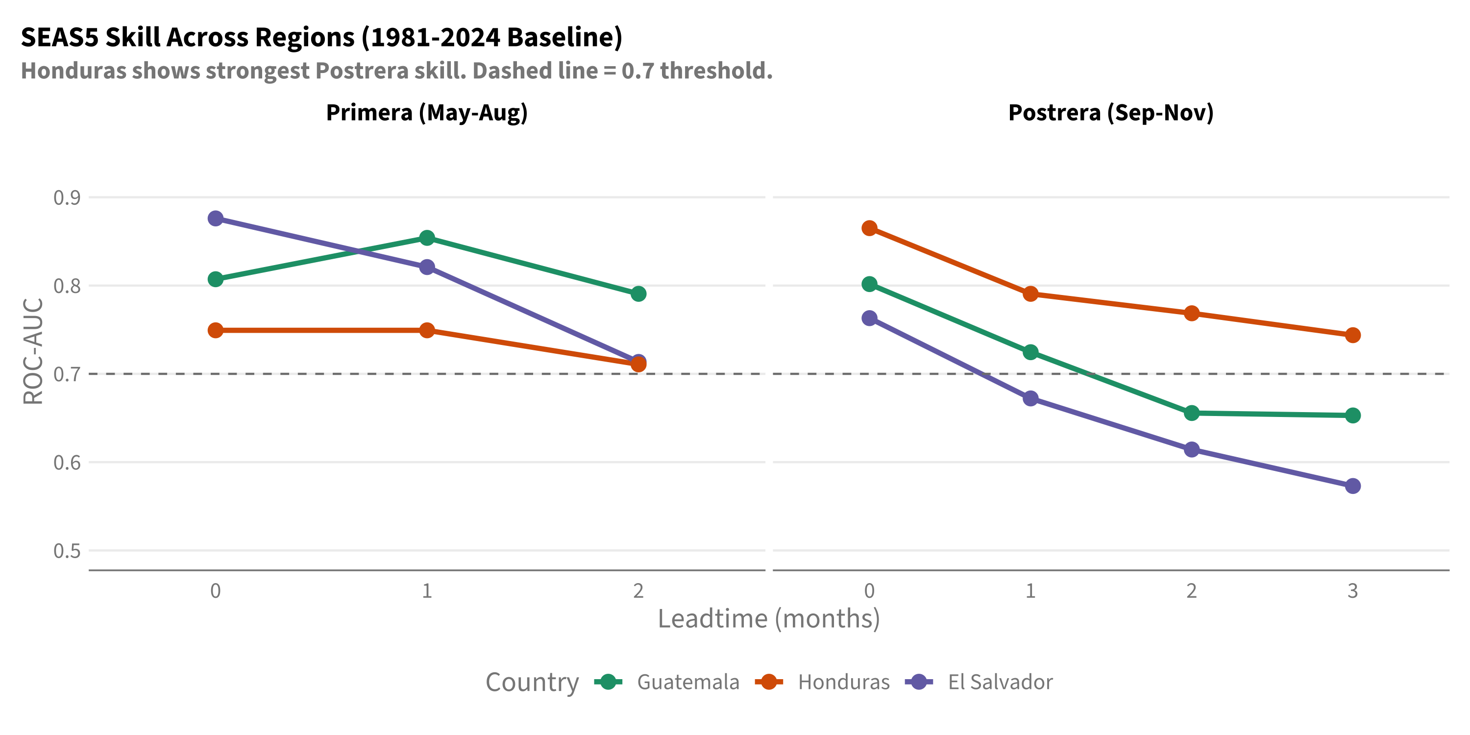
Honduras consistently shows the strongest Postrera skill, while Guatemala shows the weakest:

Code
df_skill_all |>
  filter(baseline == "1981-2024") |>
  mutate(
    window_label = factor(window,
      levels = c("primera", "postrera"),
      labels = c("Primera (May-Aug)", "Postrera (Sep-Nov)")
    )
  ) |>
  ggplot(aes(x = factor(leadtime), y = roc_auc, color = country_aoi, group = country_aoi)) +
  geom_line(linewidth = 1.2) +
  geom_point(size = 3) +
  geom_hline(yintercept = 0.7, linetype = "dashed", color = "grey50") +
  facet_wrap(~window_label, scales = "free_x") +
  scale_color_manual(values = c("Guatemala" = "#1b9e77", "Honduras" = "#d95f02", "El Salvador" = "#7570b3")) +
  scale_y_continuous(limits = c(0.5, 0.95)) +
  labs(
    title = "SEAS5 Skill Across Regions (1981-2024 Baseline)",
    subtitle = "Honduras shows strongest Postrera skill. Dashed line = 0.7 threshold.",
    x = "Leadtime (months)", y = "ROC-AUC", color = "Country"
  ) +
  theme(
    legend.position = "bottom",
    strip.text = element_text(size = 12, face = "bold"),
    plot.title = element_text(size = 14, face = "bold")
  )

7.7 Binary Performance Metrics

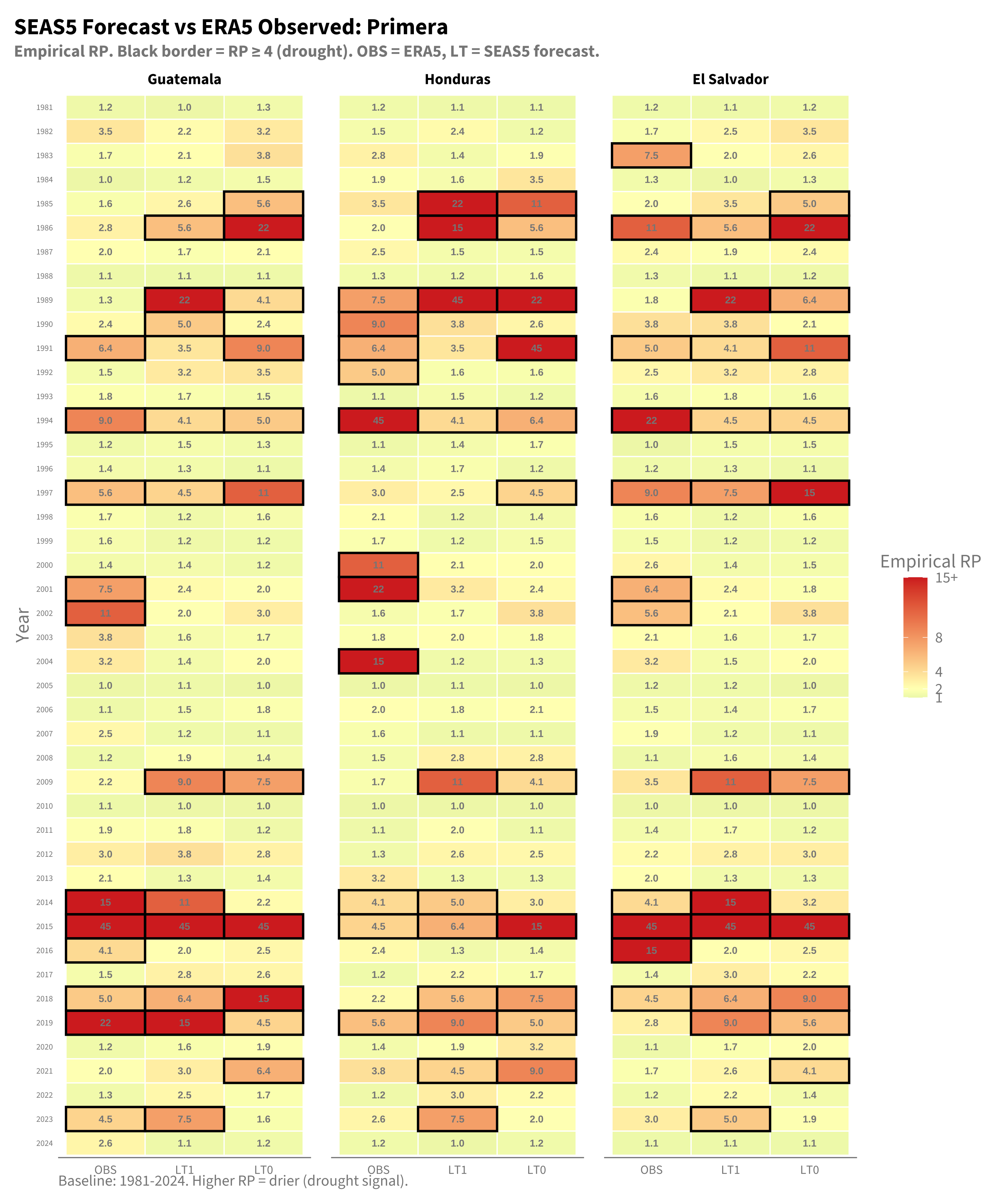
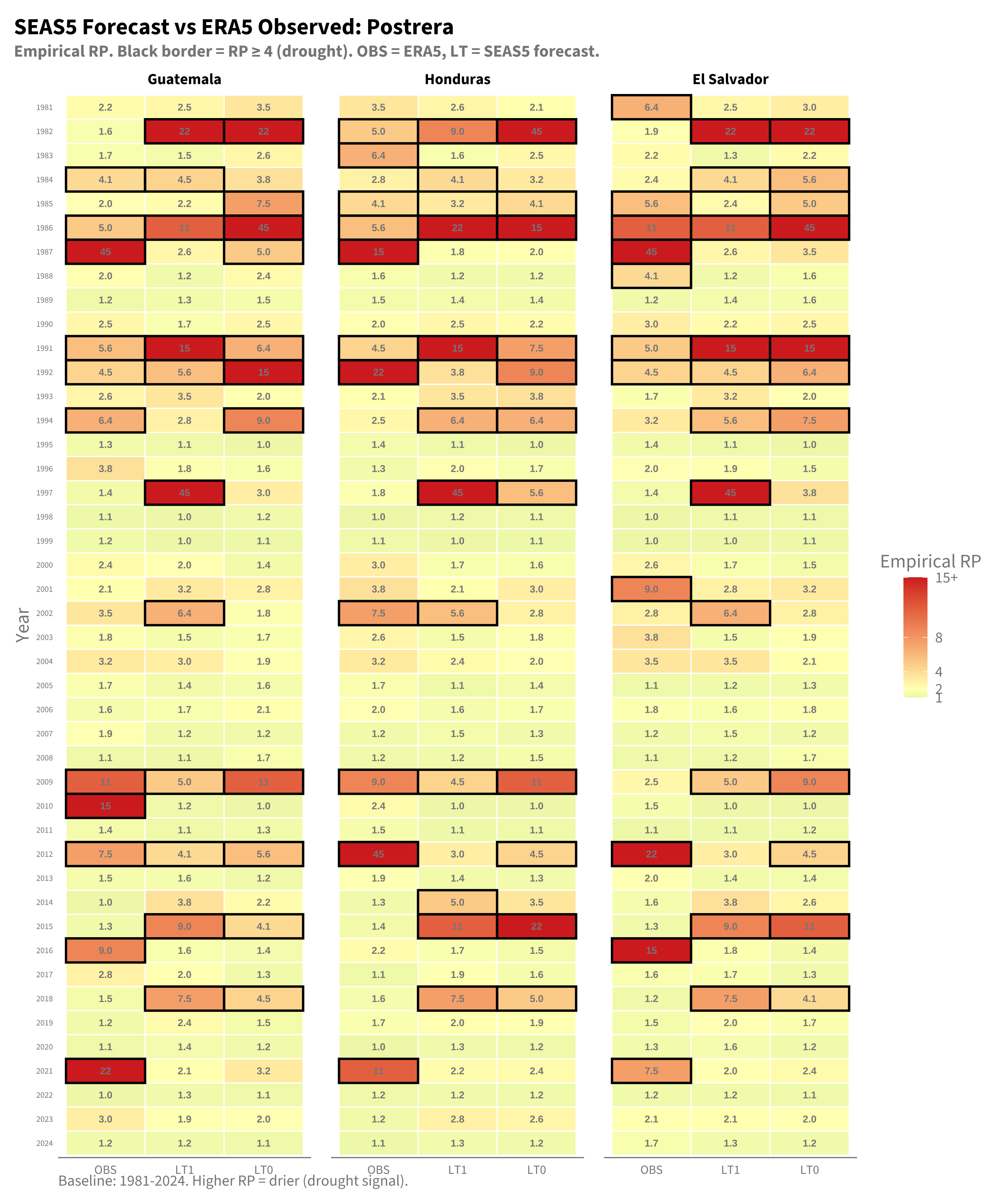
This section shows the empirical return period (RP) of both SEAS5 forecasts and ERA5 observations for each year and country, allowing direct comparison of forecast drought signals against what actually occurred.

Code
# Calculate empirical RP for forecasts
calc_empirical_rp_fcst <- function(df, baseline_start, baseline_end) {
  df |>
    filter(year >= baseline_start, year <= baseline_end) |>
    group_by(country_aoi, window, leadtime) |>
    mutate(
      n = n(),
      rank_drought = rank(fcst_mm, ties.method = "average"),
      empirical_rp = (n + 1) / rank_drought
    ) |>
    ungroup() |>
    mutate(source = paste0("LT", leadtime)) |>
    select(country_aoi, year, window, source, value_mm = fcst_mm, empirical_rp)
}

# Calculate empirical RP for observations
calc_empirical_rp_obs <- function(df, baseline_start, baseline_end) {
  df |>
    filter(year >= baseline_start, year <= baseline_end) |>
    group_by(country_aoi, window) |>
    mutate(
      n = n(),
      rank_drought = rank(obs_mm, ties.method = "average"),
      empirical_rp = (n + 1) / rank_drought
    ) |>
    ungroup() |>
    mutate(source = "OBS") |>
    select(country_aoi, year, window, source, value_mm = obs_mm, empirical_rp)
}

# Calculate RP for forecasts and observations (1981-2024 baseline)
df_rp_fcst <- calc_empirical_rp_fcst(df_joined, 1981, 2024)
df_rp_obs <- calc_empirical_rp_obs(df_obs_country, 1981, 2024)

# Combine into single dataset
df_rp_yearly <- bind_rows(df_rp_fcst, df_rp_obs)
Code
plot_yearly_rp_heatmap <- function(df, window_name, title_suffix = "") {

  df_plot <- df |>
    filter(window == window_name, source %in% c("OBS", "LT0", "LT1")) |>
    mutate(
      source = factor(source, levels = c("OBS", "LT1", "LT0")),
      country_aoi = factor(country_aoi, levels = c("Guatemala", "Honduras", "El Salvador")),
      rp_label = case_when(
        empirical_rp >= 10 ~ sprintf("%.0f", empirical_rp),
        empirical_rp >= 1 ~ sprintf("%.1f", empirical_rp),
        TRUE ~ sprintf("%.2f", empirical_rp)
      ),
      rp_capped = pmin(empirical_rp, 15)
    )

  df_drought <- df_plot |> filter(empirical_rp >= 4)

  ggplot(df_plot, aes(x = source, y = factor(year))) +
    geom_tile(aes(fill = rp_capped), color = "white", linewidth = 0.4) +
    geom_text(aes(label = rp_label), size = 2.5, fontface = "bold") +
    geom_tile(
      data = df_drought,
      aes(x = source, y = factor(year)),
      fill = NA, color = "black", linewidth = 0.8
    ) +
    facet_wrap(~country_aoi, nrow = 1) +
    scale_fill_gradient2(
      low = "#1A9850", mid = "#FFFFBF", high = "#D73027",
      midpoint = 2, limits = c(1, 15),
      name = "Empirical RP",
      oob = scales::squish,
      breaks = c(1, 2, 4, 8, 15),
      labels = c("1", "2", "4", "8", "15+")
    ) +
    scale_y_discrete(limits = rev) +
    labs(
      title = paste0("SEAS5 Forecast vs ERA5 Observed: ", str_to_title(window_name), title_suffix),
      subtitle = "Empirical RP. Black border = RP \u2265 4 (drought). OBS = ERA5, LT = SEAS5 forecast.",
      x = NULL, y = "Year",
      caption = "Baseline: 1981-2024. Higher RP = drier (drought signal)."
    ) +
    theme(
      axis.text.y = element_text(size = 6),
      axis.text.x = element_text(size = 9),
      strip.text = element_text(size = 11, face = "bold"),
      legend.position = "right",
      panel.grid = element_blank(),
      panel.spacing = unit(1, "lines"),
      plot.caption = element_text(hjust = 0)
    )
}

How to read these plots:

  • OBS: ERA5 observed rainfall (what actually happened)
  • LT1: SEAS5 forecast issued ~1 month before season start
  • LT0: SEAS5 forecast issued at season start
  • Black border: RP ≥ 4 indicates drought threshold crossed
  • Hits: Both forecast AND observation have black borders
  • False alarms: Forecast has black border but OBS doesn’t
  • Misses: OBS has black border but forecast doesn’t

7.7.1 Primera

Code
plot_yearly_rp_heatmap(df_rp_yearly, "primera")

7.7.2 Postrera

Code
plot_yearly_rp_heatmap(df_rp_yearly, "postrera")

7.7.3 F1 Score vs RP Threshold

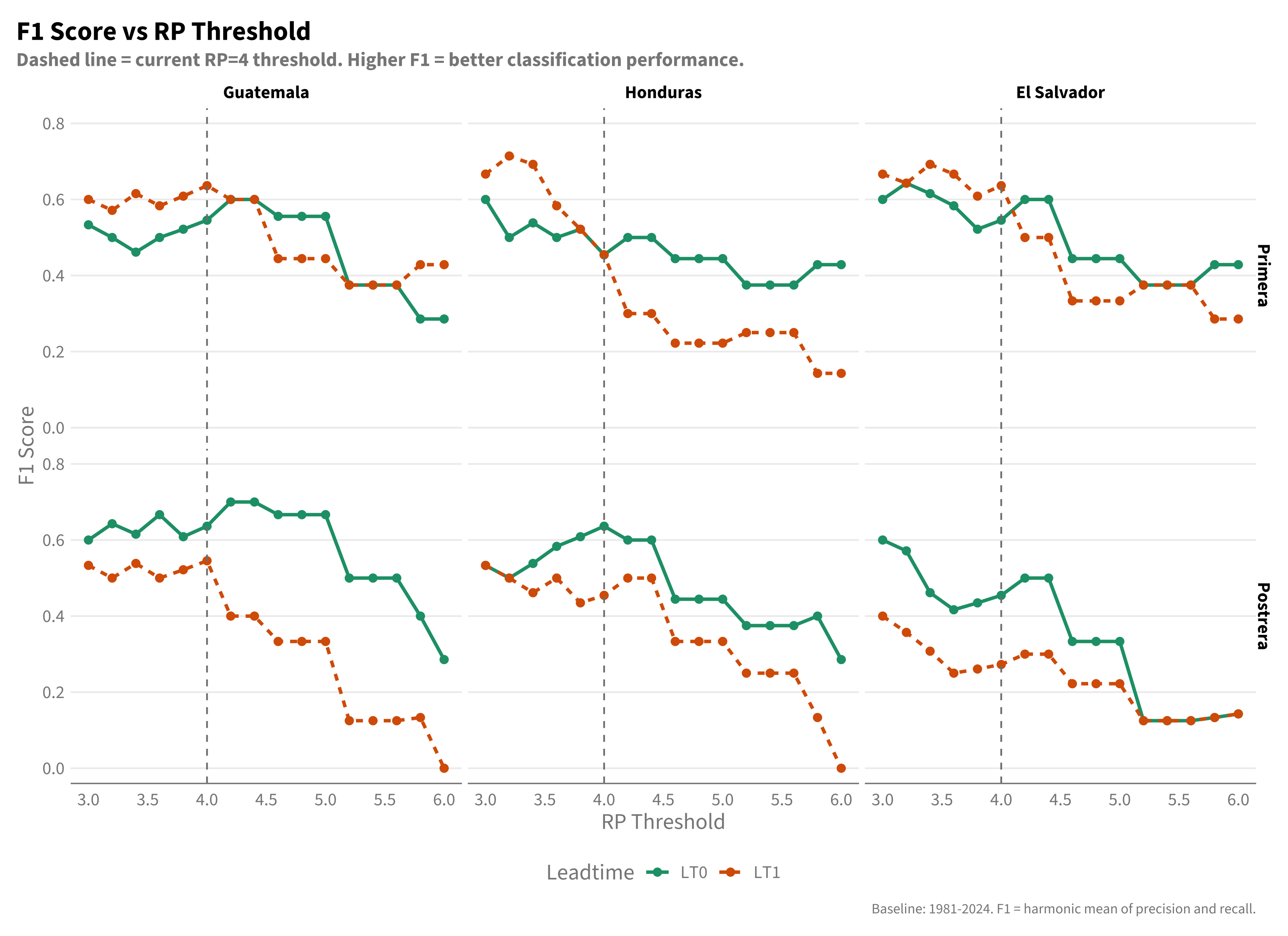
Is RP=4 the optimal threshold? This analysis shows how F1 varies as we change the drought threshold from RP=3 to RP=6.

Code
# Calculate F1 for a range of RP thresholds
rp_thresholds <- seq(3, 6, by = 0.2)

calc_f1_by_threshold <- function(df, rp_target, baseline_start = 1981, baseline_end = 2024) {
  # df_joined already has both fcst_mm and obs_mm
  df_baseline <- df |>
    filter(year >= baseline_start, year <= baseline_end)

  # Calculate obs threshold for this RP
  obs_thresholds <- df_baseline |>
    group_by(country_aoi, window) |>
    summarise(obs_thresh = calc_rp_threshold(obs_mm, rp_target, -1), .groups = "drop")

  # Calculate forecast threshold for this RP
  fcst_thresholds <- df_baseline |>
    group_by(country_aoi, window, leadtime) |>
    summarise(fcst_thresh = calc_rp_threshold(fcst_mm, rp_target, -1), .groups = "drop")

  # Classify and calculate F1
  drought_levels <- c("drought", "no_drought")

  df_baseline |>
    left_join(obs_thresholds, by = c("country_aoi", "window")) |>
    left_join(fcst_thresholds, by = c("country_aoi", "window", "leadtime")) |>
    mutate(
      truth = fct(if_else(obs_mm <= obs_thresh, "drought", "no_drought"), levels = drought_levels),
      estimate = fct(if_else(fcst_mm <= fcst_thresh, "drought", "no_drought"), levels = drought_levels)
    ) |>
    filter(!is.na(truth), !is.na(estimate)) |>
    group_by(country_aoi, window, leadtime) |>
    summarise(
      f1 = f_meas_vec(truth, estimate, event_level = "first"),
      n_drought_obs = sum(truth == "drought"),
      n_drought_fcst = sum(estimate == "drought"),
      .groups = "drop"
    ) |>
    mutate(rp_threshold = rp_target)
}

# Run for all thresholds
df_f1_by_threshold <- map_dfr(rp_thresholds, ~calc_f1_by_threshold(df_joined, .x))
Code
df_f1_by_threshold |>
  filter(leadtime %in% c(0, 1)) |>
  mutate(
    lt_label = paste0("LT", leadtime),
    country_aoi = factor(country_aoi, levels = c("Guatemala", "Honduras", "El Salvador")),
    window_label = factor(window,
      levels = c("primera", "postrera"),
      labels = c("Primera", "Postrera"))
  ) |>
  ggplot(aes(x = rp_threshold, y = f1, color = lt_label, linetype = lt_label)) +
  geom_line(linewidth = 1) +
  geom_point(size = 2) +
  geom_vline(xintercept = 4, linetype = "dashed", color = "grey50", linewidth = 0.5) +
  facet_grid(window_label ~ country_aoi) +
  scale_x_continuous(breaks = seq(3, 6, 0.5)) +
  scale_y_continuous(limits = c(0, 0.8)) +
  scale_color_manual(values = c("LT0" = "#1b9e77", "LT1" = "#d95f02")) +
  labs(
    title = "F1 Score vs RP Threshold",
    subtitle = "Dashed line = current RP=4 threshold. Higher F1 = better classification performance.",
    x = "RP Threshold",
    y = "F1 Score",
    color = "Leadtime",
    linetype = "Leadtime",
    caption = "Baseline: 1981-2024. F1 = harmonic mean of precision and recall."
  ) +
  theme(
    legend.position = "bottom",
    strip.text = element_text(size = 11, face = "bold"),
    panel.grid.minor = element_blank()
  )

Interpretation: Peaks in these curves indicate optimal thresholds. If F1 peaks at RP≠4, consider adjusting the operational threshold. Flat curves suggest the threshold choice matters less for that combination.

7.7.4 OR-Based Trigger Optimization (Postrera)

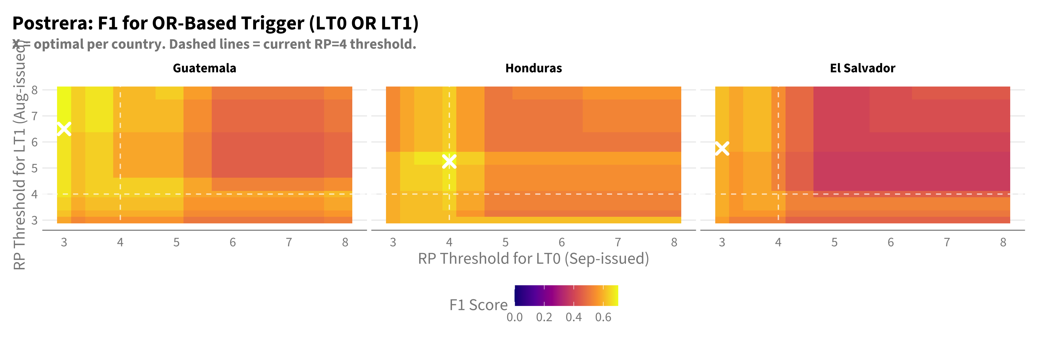
The operational trigger uses OR logic: activate if LT0 OR LT1 predicts drought. We can optimize by using different RP thresholds for each leadtime - allowing LT1 (longer lead, less accurate) to be more conservative.

Code
# Search over 2D threshold space for OR-based trigger
# Constrain both to RP >= 3 (can't go below 3 operationally)
# Expect LT0 < LT1 (LT0 more accurate, can use lower/more aggressive threshold)
rp_lt0_grid <- seq(3, 8, by = 0.25)
rp_lt1_grid <- seq(3, 8, by = 0.25)
threshold_grid <- expand.grid(rp_lt0 = rp_lt0_grid, rp_lt1 = rp_lt1_grid)

calc_or_trigger_f1 <- function(df, rp_lt0, rp_lt1, baseline_start = 1981, baseline_end = 2024) {

  df_baseline <- df |>
    filter(year >= baseline_start, year <= baseline_end, window == "postrera")

  # Get obs threshold (fixed at RP=4 - definition of drought doesn't change)
  obs_thresh_df <- df_baseline |>
    group_by(country_aoi) |>
    summarise(obs_thresh = calc_rp_threshold(obs_mm, 4, -1), .groups = "drop")

  # Get forecast thresholds per leadtime (these we optimize)
  fcst_thresh_lt0 <- df_baseline |>
    filter(leadtime == 0) |>
    group_by(country_aoi) |>
    summarise(fcst_thresh_lt0 = calc_rp_threshold(fcst_mm, rp_lt0, -1), .groups = "drop")

  fcst_thresh_lt1 <- df_baseline |>
    filter(leadtime == 1) |>
    group_by(country_aoi) |>
    summarise(fcst_thresh_lt1 = calc_rp_threshold(fcst_mm, rp_lt1, -1), .groups = "drop")

  # Pivot to wide format (one row per country-year)
  df_wide <- df_baseline |>
    filter(leadtime %in% c(0, 1)) |>
    select(country_aoi, year, leadtime, fcst_mm, obs_mm) |>
    pivot_wider(names_from = leadtime, values_from = fcst_mm, names_prefix = "fcst_lt") |>
    left_join(obs_thresh_df, by = "country_aoi") |>
    left_join(fcst_thresh_lt0, by = "country_aoi") |>
    left_join(fcst_thresh_lt1, by = "country_aoi") |>
    mutate(
      obs_drought = obs_mm <= obs_thresh,
      fcst_drought_lt0 = fcst_lt0 <= fcst_thresh_lt0,
      fcst_drought_lt1 = fcst_lt1 <= fcst_thresh_lt1,
      # OR logic: trigger if either LT predicts drought
      fcst_drought_or = fcst_drought_lt0 | fcst_drought_lt1
    )

  # Calculate F1 per country using yardstick
  drought_levels <- c("drought", "no_drought")

  df_wide |>
    mutate(
      truth = fct(if_else(obs_drought, "drought", "no_drought"), levels = drought_levels),
      estimate = fct(if_else(fcst_drought_or, "drought", "no_drought"), levels = drought_levels)
    ) |>
    group_by(country_aoi) |>
    summarise(
      f1 = f_meas_vec(truth, estimate, event_level = "first"),
      precision = precision_vec(truth, estimate, event_level = "first"),
      recall = recall_vec(truth, estimate, event_level = "first"),
      .groups = "drop"
    ) |>
    mutate(rp_lt0 = rp_lt0, rp_lt1 = rp_lt1)
}

# Run grid search
df_or_grid <- map2_dfr(
  threshold_grid$rp_lt0,
  threshold_grid$rp_lt1,
  ~calc_or_trigger_f1(df_joined, .x, .y)
)

7.7.4.1 F1 by Country

Code
# Find optimal per country
df_optimal_country <- df_or_grid |>
  group_by(country_aoi) |>
  slice_max(f1, n = 1) |>
  slice(1)

df_or_grid |>
  mutate(country_aoi = factor(country_aoi, levels = c("Guatemala", "Honduras", "El Salvador"))) |>
  ggplot(aes(x = rp_lt0, y = rp_lt1, fill = f1)) +
  geom_tile() +
  geom_point(data = df_optimal_country |>
               mutate(country_aoi = factor(country_aoi, levels = c("Guatemala", "Honduras", "El Salvador"))),
             color = "white", size = 3, shape = 4, stroke = 2) +
  geom_vline(xintercept = 4, linetype = "dashed", color = "white", alpha = 0.7) +
  geom_hline(yintercept = 4, linetype = "dashed", color = "white", alpha = 0.7) +
  facet_wrap(~country_aoi) +
  scale_fill_viridis_c(option = "plasma", limits = c(0, 0.7), na.value = "grey50") +
  labs(
    title = "Postrera: F1 for OR-Based Trigger (LT0 OR LT1)",
    subtitle = "X = optimal per country. Dashed lines = current RP=4 threshold.",
    x = "RP Threshold for LT0 (Sep-issued)",
    y = "RP Threshold for LT1 (Aug-issued)",
    fill = "F1 Score"
  ) +
  theme(
    strip.text = element_text(size = 11, face = "bold")
  )

7.7.4.2 Average F1 Across Countries

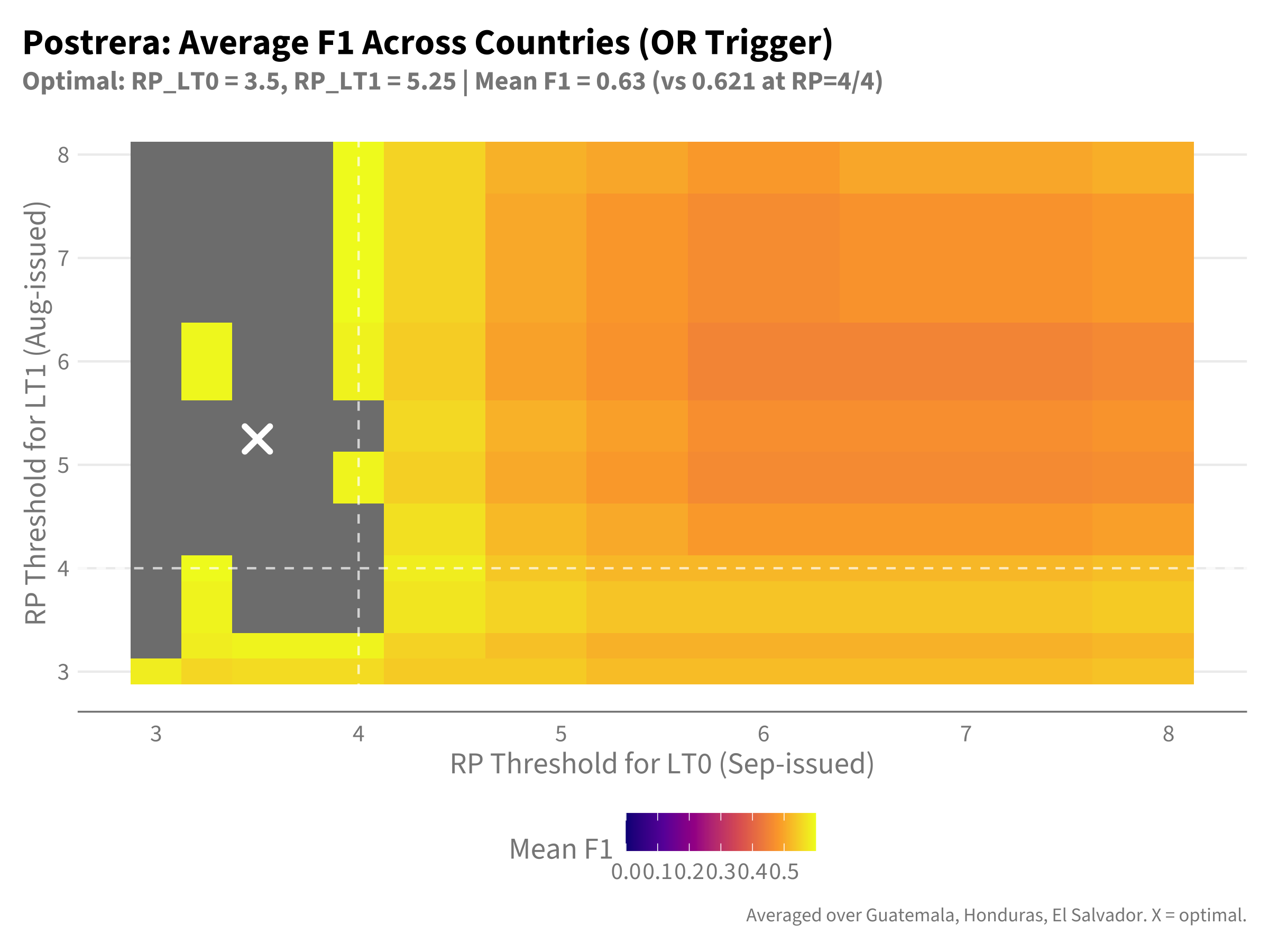
For a single operational threshold, we average F1 across all three countries.

Code
# Average F1 across all countries for each threshold combination
df_or_avg <- df_or_grid |>
  group_by(rp_lt0, rp_lt1) |>
  summarise(
    f1_mean = mean(f1, na.rm = TRUE),
    f1_min = min(f1, na.rm = TRUE),
    f1_max = max(f1, na.rm = TRUE),
    .groups = "drop"
  )

# Find overall optimal
df_optimal_overall <- df_or_avg |>
  slice_max(f1_mean, n = 1) |>
  slice(1)

# Baseline F1 at RP=4/RP=4
f1_baseline <- df_or_avg |>
  filter(rp_lt0 == 4, rp_lt1 == 4) |>
  pull(f1_mean)

ggplot(df_or_avg, aes(x = rp_lt0, y = rp_lt1, fill = f1_mean)) +
  geom_tile() +
  geom_point(data = df_optimal_overall, color = "white", size = 4, shape = 4, stroke = 2) +
  geom_vline(xintercept = 4, linetype = "dashed", color = "white", alpha = 0.7) +
  geom_hline(yintercept = 4, linetype = "dashed", color = "white", alpha = 0.7) +
  scale_fill_viridis_c(option = "plasma", limits = c(0, 0.6), na.value = "grey50") +
  labs(
    title = "Postrera: Average F1 Across Countries (OR Trigger)",
    subtitle = paste0("Optimal: RP_LT0 = ", df_optimal_overall$rp_lt0,
                      ", RP_LT1 = ", df_optimal_overall$rp_lt1,
                      " | Mean F1 = ", round(df_optimal_overall$f1_mean, 3),
                      " (vs ", round(f1_baseline, 3), " at RP=4/4)"),
    x = "RP Threshold for LT0 (Sep-issued)",
    y = "RP Threshold for LT1 (Aug-issued)",
    fill = "Mean F1",
    caption = "Averaged over Guatemala, Honduras, El Salvador. X = optimal."
  )

7.7.4.3 Summary Table

Code
# Get baseline F1 per country at RP=4/RP=4
df_baseline_f1 <- df_or_grid |>
  filter(rp_lt0 == 4, rp_lt1 == 4) |>
  select(country_aoi, f1_baseline = f1)

# Function to calculate empirical combined RP for OR trigger
calc_empirical_or_rp <- function(df, rp_lt0, rp_lt1, baseline_start = 1981, baseline_end = 2024) {
  df_baseline <- df |>
    filter(year >= baseline_start, year <= baseline_end, window == "postrera")

  # Get forecast thresholds per leadtime
 fcst_thresh_lt0 <- df_baseline |>
    filter(leadtime == 0) |>
    group_by(country_aoi) |>
    summarise(fcst_thresh_lt0 = calc_rp_threshold(fcst_mm, rp_lt0, -1), .groups = "drop")

  fcst_thresh_lt1 <- df_baseline |>
    filter(leadtime == 1) |>
    group_by(country_aoi) |>
    summarise(fcst_thresh_lt1 = calc_rp_threshold(fcst_mm, rp_lt1, -1), .groups = "drop")

  # Pivot and calculate OR trigger
  df_baseline |>
    filter(leadtime %in% c(0, 1)) |>
    select(country_aoi, year, leadtime, fcst_mm) |>
    pivot_wider(names_from = leadtime, values_from = fcst_mm, names_prefix = "fcst_lt") |>
    left_join(fcst_thresh_lt0, by = "country_aoi") |>
    left_join(fcst_thresh_lt1, by = "country_aoi") |>
    mutate(
      fcst_drought_lt0 = fcst_lt0 <= fcst_thresh_lt0,
      fcst_drought_lt1 = fcst_lt1 <= fcst_thresh_lt1,
      fcst_drought_or = fcst_drought_lt0 | fcst_drought_lt1
    ) |>
    group_by(country_aoi) |>
    summarise(
      n_years = n(),
      n_triggers = sum(fcst_drought_or, na.rm = TRUE),
      rp_empirical = (n_years + 1) / n_triggers,
      .groups = "drop"
    )
}

# Get empirical RP for each threshold combo in the optimal set
df_rp_country <- map2_dfr(
  df_optimal_country$rp_lt0,
  df_optimal_country$rp_lt1,
  ~calc_empirical_or_rp(df_joined, .x, .y) |>
    mutate(rp_lt0 = .x, rp_lt1 = .y)
)

df_rp_overall <- calc_empirical_or_rp(df_joined, df_optimal_overall$rp_lt0, df_optimal_overall$rp_lt1) |>
  mutate(rp_lt0 = df_optimal_overall$rp_lt0, rp_lt1 = df_optimal_overall$rp_lt1)

df_rp_baseline <- calc_empirical_or_rp(df_joined, 4, 4)

# Country-specific optima
df_country_summary <- df_optimal_country |>
  left_join(df_baseline_f1, by = "country_aoi") |>
  left_join(df_rp_country |> select(country_aoi, rp_lt0, rp_lt1, rp_empirical),
            by = c("country_aoi", "rp_lt0", "rp_lt1")) |>
  mutate(
    f1_improvement = f1 - f1_baseline,
    type = "Country-specific"
  ) |>
  select(type, country_aoi, rp_lt0, rp_lt1, rp_empirical, f1, f1_baseline, f1_improvement)

# Overall optimum applied to each country
df_overall_applied <- df_or_grid |>
  filter(rp_lt0 == df_optimal_overall$rp_lt0, rp_lt1 == df_optimal_overall$rp_lt1) |>
  left_join(df_baseline_f1, by = "country_aoi") |>
  left_join(df_rp_overall |> select(country_aoi, rp_empirical), by = "country_aoi") |>
  mutate(
    f1_improvement = f1 - f1_baseline,
    type = "Overall optimal"
  ) |>
  select(type, country_aoi, rp_lt0, rp_lt1, rp_empirical, f1, f1_baseline, f1_improvement)

# Get average baseline empirical RP
rp_baseline_avg <- mean(df_rp_baseline$rp_empirical)

bind_rows(df_overall_applied, df_country_summary) |>
  mutate(type = factor(type, levels = c("Overall optimal", "Country-specific"))) |>
  arrange(type, country_aoi) |>
  gt() |>
  fmt_number(columns = c(rp_lt0, rp_lt1, rp_empirical), decimals = 2) |>
  fmt_number(columns = c(f1, f1_baseline, f1_improvement), decimals = 3) |>
  cols_label(
    type = "Optimization",
    country_aoi = "Country",
    rp_lt0 = "RP (LT0)",
    rp_lt1 = "RP (LT1)",
    rp_empirical = "RP (OR)",
    f1 = "F1",
    f1_baseline = "Baseline F1",
    f1_improvement = "Δ F1"
  ) |>
  tab_header(
    title = "OR-Trigger Threshold Optimization Results",
    subtitle = sprintf("Baseline = RP=4/4 (empirical OR RP ≈ %.1f)", rp_baseline_avg)
  ) |>
  tab_style(
    style = cell_fill(color = "#d4edda"),
    locations = cells_body(columns = f1_improvement, rows = f1_improvement > 0)
  ) |>
  tab_row_group(
    label = md("**Overall Optimal Thresholds**"),
    rows = type == "Overall optimal"
  ) |>
  tab_row_group(
    label = md("**Country-Specific Optimal Thresholds**"),
    rows = type == "Country-specific"
  ) |>
  cols_hide(type)
OR-Trigger Threshold Optimization Results
Baseline = RP=4/4 (empirical OR RP ≈ 3.3)
Country RP (LT0) RP (LT1) RP (OR) F1 Baseline F1 Δ F1
Country-Specific Optimal Thresholds
El Salvador 3.00 5.75 2.81 0.615 0.583 0.032
Guatemala 3.00 6.50 3.00 0.692 0.640 0.052
Honduras 4.00 5.25 3.75 0.696 0.640 0.056
Overall Optimal Thresholds
El Salvador 3.50 5.25 3.46 0.583 0.583 0.000
Guatemala 3.50 5.25 3.21 0.640 0.640 0.000
Honduras 3.50 5.25 3.46 0.667 0.640 0.027

Optimal Thresholds Summary:

Code
# Print the key numbers
cat("Overall Optimal (averaged across countries):\n")
Overall Optimal (averaged across countries):
Code
cat(sprintf("  LT0 (Sep): RP = %.2f\n", df_optimal_overall$rp_lt0))
  LT0 (Sep): RP = 3.50
Code
cat(sprintf("  LT1 (Aug): RP = %.2f\n", df_optimal_overall$rp_lt1))
  LT1 (Aug): RP = 5.25
Code
cat(sprintf("  Empirical OR RP = %.2f (vs %.2f at RP=4/4)\n",
            mean(df_rp_overall$rp_empirical), rp_baseline_avg))
  Empirical OR RP = 3.38 (vs 3.30 at RP=4/4)
Code
cat(sprintf("  Mean F1 = %.3f (vs %.3f at RP=4/4)\n\n", df_optimal_overall$f1_mean, f1_baseline))
  Mean F1 = 0.630 (vs 0.621 at RP=4/4)
Code
cat("Country-Specific Optimal:\n")
Country-Specific Optimal:
Code
df_optimal_country |>
  left_join(df_rp_country |> select(country_aoi, rp_lt0, rp_lt1, rp_empirical),
            by = c("country_aoi", "rp_lt0", "rp_lt1")) |>
  arrange(country_aoi) |>
  rowwise() |>
  mutate(msg = sprintf("  %s: LT0=%.2f, LT1=%.2f, OR RP=%.2f (F1=%.3f)",
                       country_aoi, rp_lt0, rp_lt1, rp_empirical, f1)) |>
  pull(msg) |>
  cat(sep = "\n")
  El Salvador: LT0=3.00, LT1=5.75, OR RP=2.81 (F1=0.615)
  Guatemala: LT0=3.00, LT1=6.50, OR RP=3.00 (F1=0.692)
  Honduras: LT0=4.00, LT1=5.25, OR RP=3.75 (F1=0.696)

7.8 Summary Table

Code
# Create summary table for 1981 baseline with recommendations
df_summary <- df_skill_all |>
  filter(baseline == "1981-2024") |>
  filter(
    (window == "primera" & leadtime %in% 0:2) |
    (window == "postrera" & leadtime %in% 0:3)
  ) |>
  mutate(
    score = sprintf("%.2f (%.2f)", roc_auc, f1),
    lt_label = paste0("LT", leadtime),
    # Format window labels with months
    window = case_when(
      window == "primera" ~ "Primera (May-Aug)",
      window == "postrera" ~ "Postrera (Sep-Nov)"
    ),
    # Flag recommended combinations
    recommended = case_when(
      window == "Primera (May-Aug)" & leadtime %in% 0:2 ~ TRUE,
      window == "Postrera (Sep-Nov)" & leadtime %in% 0:1 ~ TRUE,
      TRUE ~ FALSE
    )
  ) |>
  select(country_aoi, window, lt_label, score, roc_auc, recommended) |>
  pivot_wider(names_from = lt_label, values_from = c(score, roc_auc, recommended))

# Build GT table
df_summary |>
  select(country_aoi, window, starts_with("score_")) |>
  rename_with(~str_remove(.x, "score_"), starts_with("score_")) |>
  gt(groupname_col = "window") |>
  tab_header(
    title = md("**SEAS5 Forecast Skill: ROC-AUC (F1)**"),
    subtitle = md("RP4 drought threshold | 1981-2024 baseline | *Recommended leadtimes highlighted*")
  ) |>
  cols_label(country_aoi = "Country") |>
  tab_style(
    style = list(
      cell_fill(color = "#c7e9c0"),
      cell_text(weight = "bold")
    ),
    locations = list(
      cells_body(columns = c(LT0, LT1, LT2), rows = window == "Primera (May-Aug)"),
      cells_body(columns = c(LT0, LT1), rows = window == "Postrera (Sep-Nov)")
    )
  ) |>
  tab_style(
    style = cell_text(color = "#6c757d"),
    locations = cells_body(columns = c(LT2, LT3), rows = window == "Postrera (Sep-Nov)")
  ) |>
  tab_style(
    style = cell_text(weight = "bold", size = px(13)),
    locations = cells_row_groups()
  ) |>
  tab_style(
    style = cell_borders(sides = "bottom", color = "#dee2e6", weight = px(2)),
    locations = cells_column_labels()
  ) |>
  tab_footnote(
    footnote = md("**Green** = recommended for operational use; Gray = use with caution"),
    locations = cells_title(groups = "subtitle")
  ) |>
  tab_footnote(
    footnote = "Format: ROC-AUC (F1). ROC-AUC > 0.7 = good; > 0.8 = excellent",
    locations = cells_column_labels(columns = LT0)
  ) |>
  tab_source_note(
    source_note = md("**Recommendation**: Use LT0-2 for Primera, LT0-1 for Postrera. Honduras shows strongest Postrera skill.")
  ) |>
  tab_options(
    table.font.size = px(14),
    heading.title.font.size = px(18),
    heading.subtitle.font.size = px(13),
    column_labels.font.weight = "bold",
    row_group.background.color = "#f8f9fa",
    table.border.top.style = "solid",
    table.border.top.width = px(2),
    table.border.top.color = "#1a9850"
  )

SEAS5 Forecast Skill Summary

SEAS5 Forecast Skill: ROC-AUC (F1)
RP4 drought threshold | 1981-2024 baseline | Recommended leadtimes highlighted1
Country LT02 LT1 LT2 LT3
Postrera (Sep-Nov)
El Salvador 0.76 (0.45) 0.67 (0.27) 0.61 (0.27) 0.57 (0.36)
Guatemala 0.80 (0.64) 0.72 (0.55) 0.66 (0.36) 0.65 (0.45)
Honduras 0.87 (0.64) 0.79 (0.45) 0.77 (0.55) 0.74 (0.36)
Primera (May-Aug)
El Salvador 0.88 (0.55) 0.82 (0.64) 0.71 (0.55) NA
Guatemala 0.81 (0.55) 0.85 (0.64) 0.79 (0.64) NA
Honduras 0.75 (0.45) 0.75 (0.45) 0.71 (0.55) NA
Recommendation: Use LT0-2 for Primera, LT0-1 for Postrera. Honduras shows strongest Postrera skill.
1 Green = recommended for operational use; Gray = use with caution
2 Format: ROC-AUC (F1). ROC-AUC > 0.7 = good; > 0.8 = excellent

7.9 Tolerant F1: Accounting for Near-Miss Events

Standard F1 score uses a strict binary classification: both the forecast and observation must cross the exact same RP4 threshold for a True Positive. This is harsh because forecasting drought when a “pretty dry” year occurred (e.g., RP3.5) receives zero credit.

The problem with strict F1:

Consider a year where:

  • Forecast: drought (below RP4 threshold)
  • Observation: RP3.5 (dry, but just above RP4 threshold)

Under strict rules, this is a False Positive. But operationally, this forecast was useful - it correctly identified a dry year.

Asymmetric tolerance approach:

We define three observation categories:

  • Severe drought: obs ≤ RP4 threshold (~25% of years)
  • Marginal: RP4 < obs ≤ RP3 (~8% of years, the “buffer zone”)
  • Normal: obs > RP3 (~67% of years)

The asymmetric rules:

  • TP: Forecast drought AND observation is severe OR marginal (give credit for “close enough”)
  • FP: Forecast drought AND observation is normal (only penalize if clearly not drought)
  • FN: No forecast AND observation is severe (only penalize misses of clear droughts)
  • TN: No forecast AND observation is marginal OR normal

This approach treats marginal years favorably in both directions: forecast drought gets credit, no-forecast isn’t penalized.

Code
# Calculate thresholds for both RP levels
calc_rp_threshold <- function(x, rp_target = 4, direction = -1) {
  x <- x[!is.na(x)]
  n <- length(x)
  if (n < 3) return(NA_real_)
  ranks <- rank(x * -direction, ties.method = "average")
  rp <- (n + 1) / ranks
  approx(rp, x, xout = rp_target, rule = 2)$y
}

# Get thresholds
obs_thresholds_dual <- df_joined |>
  filter(year >= 1981, year <= 2024) |>
  group_by(country_aoi, window) |>
  summarise(
    obs_thresh_rp4 = calc_rp_threshold(obs_mm, 4, -1),
    obs_thresh_rp3 = calc_rp_threshold(obs_mm, 3, -1),
    .groups = "drop"
  )

fcst_thresholds <- df_joined |>
  filter(year >= 1981, year <= 2024) |>
  group_by(country_aoi, window, leadtime) |>
  summarise(fcst_thresh = calc_rp_threshold(fcst_mm, 4, -1), .groups = "drop")

# Calculate both strict and tolerant F1
df_f1_comparison <- df_joined |>
  filter(year >= 1981, year <= 2024) |>
  left_join(obs_thresholds_dual, by = c("country_aoi", "window")) |>
  left_join(fcst_thresholds, by = c("country_aoi", "window", "leadtime")) |>
  mutate(fcst_drought = fcst_mm <= fcst_thresh) |>
  group_by(country_aoi, window, leadtime) |>
  summarise(
    # Strict F1
    strict_tp = sum(fcst_drought & obs_mm <= obs_thresh_rp4),
    strict_fp = sum(fcst_drought & obs_mm > obs_thresh_rp4),
    strict_fn = sum(!fcst_drought & obs_mm <= obs_thresh_rp4),
    f1_strict = 2 * strict_tp / (2 * strict_tp + strict_fp + strict_fn),

    # Tolerant F1 (asymmetric)
    tol_tp = sum(fcst_drought & obs_mm <= obs_thresh_rp3),
    tol_fp = sum(fcst_drought & obs_mm > obs_thresh_rp3),
    tol_fn = sum(!fcst_drought & obs_mm <= obs_thresh_rp4),
    f1_tolerant = 2 * tol_tp / (2 * tol_tp + tol_fp + tol_fn),

    .groups = "drop"
  ) |>
  mutate(
    improvement = f1_tolerant - f1_strict,
    country_aoi = factor(country_aoi, levels = c("Guatemala", "Honduras", "El Salvador")),
    window = factor(window, levels = c("primera", "postrera"))
  )
Code
df_f1_comparison |>
  filter(leadtime %in% 0:2) |>
  mutate(
    comparison = sprintf("%.2f → %.2f", f1_strict, f1_tolerant)
  ) |>
  select(country_aoi, window, leadtime, comparison) |>
  pivot_wider(names_from = leadtime, values_from = comparison, names_prefix = "LT") |>
  arrange(window, country_aoi) |>
  gt(groupname_col = "window") |>
  tab_header(
    title = md("**F1 Score: Strict → Tolerant**"),
    subtitle = "Tolerant F1 gives credit when forecast drought aligns with marginal (RP3-4) years"
  ) |>
  cols_label(country_aoi = "Country") |>
  tab_style(
    style = cell_text(weight = "bold"),
    locations = cells_row_groups()
  ) |>
  tab_footnote(
    footnote = "Tolerant F1 never decreases - marginal years count as TP if forecast drought, TN if not",
    locations = cells_title(groups = "subtitle")
  )
F1 Score Comparison: Strict vs Tolerant
F1 Score: Strict → Tolerant
Tolerant F1 gives credit when forecast drought aligns with marginal (RP3-4) years1
Country LT0 LT1 LT2
primera
Guatemala 0.55 → 0.55 0.64 → 0.64 0.64 → 0.64
Honduras 0.45 → 0.64 0.45 → 0.58 0.55 → 0.61
El Salvador 0.55 → 0.61 0.64 → 0.75 0.55 → 0.67
postrera
Guatemala 0.64 → 0.64 0.55 → 0.61 0.36 → 0.50
Honduras 0.64 → 0.64 0.45 → 0.45 0.55 → 0.55
El Salvador 0.45 → 0.52 0.27 → 0.35 0.27 → 0.35
1 Tolerant F1 never decreases - marginal years count as TP if forecast drought, TN if not
Code
df_f1_comparison |>
  filter(leadtime %in% 0:2) |>
  ggplot(aes(x = factor(leadtime), y = improvement, fill = country_aoi)) +
  geom_col(position = position_dodge(width = 0.8), width = 0.7) +
  geom_hline(yintercept = 0, linetype = "dashed", color = "grey50") +
  facet_wrap(~window, labeller = labeller(window = c(primera = "Primera (May-Aug)", postrera = "Postrera (Sep-Nov)"))) +
  scale_fill_manual(values = c("Guatemala" = "#1b9e77", "Honduras" = "#d95f02", "El Salvador" = "#7570b3")) +
  scale_y_continuous(labels = scales::percent_format(accuracy = 1), limits = c(0, 0.25)) +
  labs(
    title = "F1 Improvement with Tolerant Scoring",
    subtitle = "Marginal years (RP3-4) count as TP if forecast drought, TN if no forecast",
    x = "Leadtime", y = "F1 Improvement", fill = "Country"
  ) +
  theme(
    legend.position = "bottom",
    strip.text = element_text(size = 12, face = "bold")
  )

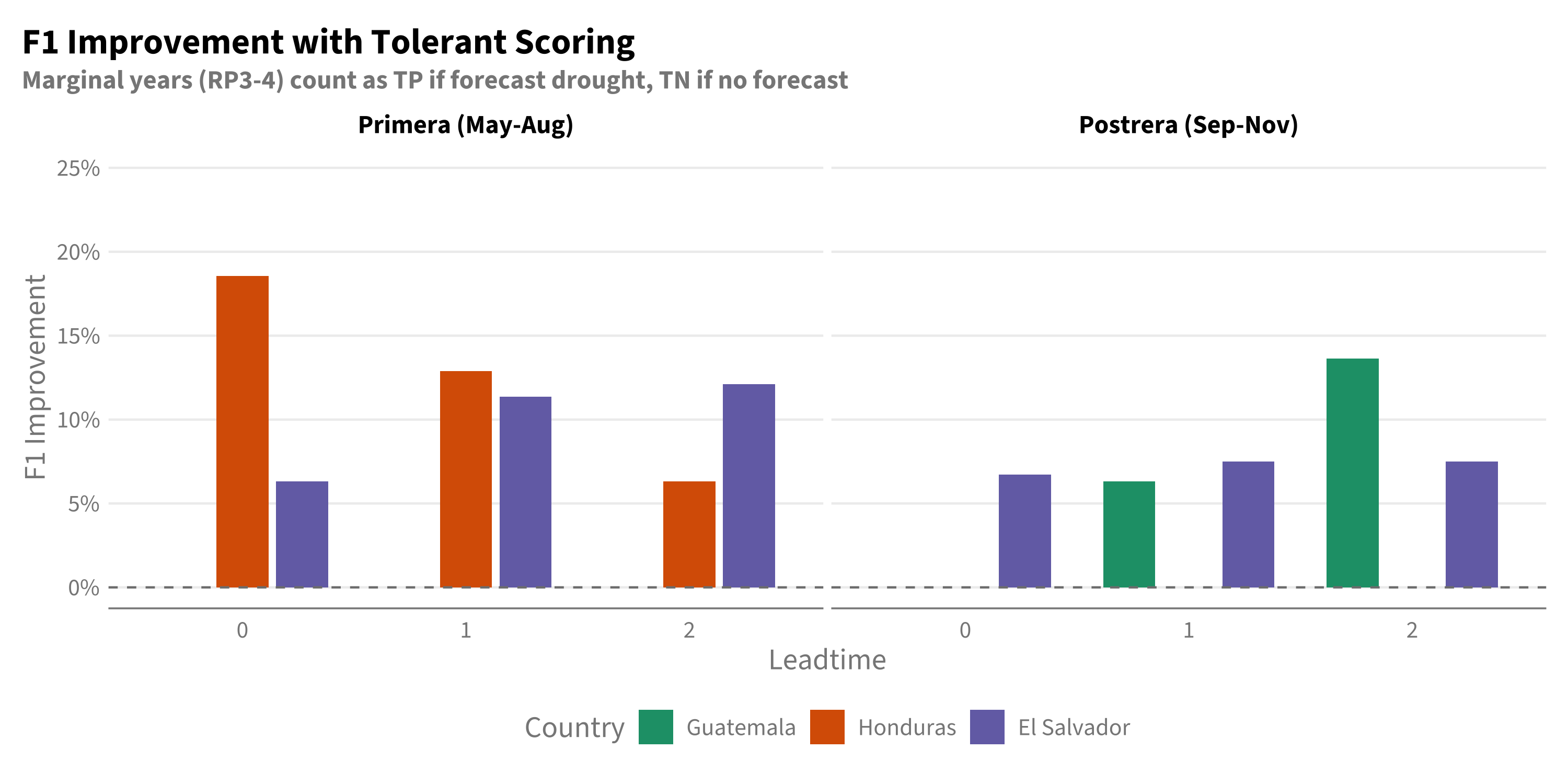
F1 improvement from tolerant scoring. Bars show the increase in F1 when marginal (RP3-4) years are treated favorably.

Key findings:

  • Tolerant F1 never decreases compared to strict F1 (all improvements ≥ 0)
  • Mean F1 improves from 0.51 to 0.58 (+15% relative)
  • Honduras and El Salvador Primera show the largest gains (+0.13 to +0.19)
  • Guatemala shows minimal change in some cases - the forecast false positives were truly normal years, not marginal

Interpretation: The tolerant metric rewards forecasts that correctly identify “dry-ish” years, while maintaining strict standards for detecting severe droughts. This better reflects operational value: a drought forecast followed by a moderately dry year is more useful than it appears under strict scoring.

7.10 Combined Annual Return Period

When using multiple leadtimes and both seasons, the effective annual trigger frequency is higher than the per-forecast RP4 threshold suggests. If any forecast in any season crosses the RP4 threshold, you trigger - and with multiple “chances” per year, triggers become more frequent.

The math: If each forecast has independent 25% trigger probability (RP4), the probability of triggering at least once across N forecasts is:

\[P(\text{at least one trigger}) = 1 - (1 - 0.25)^N\]

With 3 Primera leadtimes (LT0-2) and 2 Postrera leadtimes (LT0-1), that’s 5 forecasts per year, giving a theoretical combined RP of ~1.8 years if forecasts were independent. But forecasts are correlated (especially within-season), so the actual combined RP will be higher.

Code
# Calculate trigger flags for each forecast
df_triggers <- df_joined |>
  filter(year >= 1981, year <= 2024) |>
  left_join(
    # Forecast thresholds (RP4)
    df_joined |>
      filter(year >= 1981, year <= 2024) |>
      group_by(country_aoi, window, leadtime) |>
      summarise(fcst_thresh = calc_rp_threshold(fcst_mm, 4, -1), .groups = "drop"),
    by = c("country_aoi", "window", "leadtime")
  ) |>
  mutate(triggered = fcst_mm <= fcst_thresh)

# Per-season combined RP (any LT in that season)
df_rp_by_season <- df_triggers |>
  filter(
    (window == "primera" & leadtime %in% 0:2) |
    (window == "postrera" & leadtime %in% 0:1)
  ) |>
  group_by(country_aoi, window, year) |>
  summarise(triggered_season = any(triggered), .groups = "drop") |>
  group_by(country_aoi, window) |>
  summarise(
    n_years = n(),
    n_triggered = sum(triggered_season),
    trigger_rate = mean(triggered_season),
    combined_rp = 1 / trigger_rate,
    .groups = "drop"
  )

# Annual combined RP (any LT in either season)
df_rp_annual <- df_triggers |>
  filter(
    (window == "primera" & leadtime %in% 0:2) |
    (window == "postrera" & leadtime %in% 0:1)
  ) |>
  group_by(country_aoi, year) |>
  summarise(triggered_annual = any(triggered), .groups = "drop") |>
  group_by(country_aoi) |>
  summarise(
    n_years = n(),
    n_triggered = sum(triggered_annual),
    trigger_rate = mean(triggered_annual),
    combined_rp = 1 / trigger_rate,
    .groups = "drop"
  )
Code
# Format for display
df_rp_display <- df_rp_by_season |>
  mutate(
    window = case_when(
      window == "primera" ~ "Primera (LT0-2)",
      window == "postrera" ~ "Postrera (LT0-1)"
    ),
    display = sprintf("%.1f yr (%d/%d)", combined_rp, n_triggered, n_years)
  ) |>
  select(country_aoi, window, display) |>
  pivot_wider(names_from = window, values_from = display)

df_annual_display <- df_rp_annual |>
  mutate(
    `Annual (Either Season)` = sprintf("%.1f yr (%d/%d)", combined_rp, n_triggered, n_years)
  ) |>
  select(country_aoi, `Annual (Either Season)`)

df_rp_display |>
  left_join(df_annual_display, by = "country_aoi") |>
  gt() |>
  tab_header(
    title = md("**Combined Trigger Return Period**"),
    subtitle = "RP4 threshold at each leadtime | 1981-2024 baseline"
  ) |>
  cols_label(country_aoi = "Country") |>
  tab_footnote(
    footnote = "Format: Combined RP (years triggered / total years)",
    locations = cells_column_labels(columns = `Primera (LT0-2)`)
  ) |>
  tab_source_note(
    source_note = "Combined RP = 1 / (proportion of years with at least one trigger)"
  )

Combined Return Period by Season and Annual

Combined Trigger Return Period
RP4 threshold at each leadtime | 1981-2024 baseline
Country Postrera (LT0-1) Primera (LT0-2)1 Annual (Either Season)
El Salvador 3.4 yr (13/44) 2.9 yr (15/44) 2.3 yr (19/44)
Guatemala 3.1 yr (14/44) 3.1 yr (14/44) 2.2 yr (20/44)
Honduras 3.1 yr (14/44) 2.9 yr (15/44) 2.2 yr (20/44)
Combined RP = 1 / (proportion of years with at least one trigger)
1 Format: Combined RP (years triggered / total years)
Code
bind_rows(
  df_rp_by_season |>
    mutate(scope = if_else(window == "primera", "Primera (LT0-2)", "Postrera (LT0-1)")),
  df_rp_annual |>
    mutate(scope = "Annual (Either)")
) |>
  mutate(
    scope = factor(scope, levels = c("Primera (LT0-2)", "Postrera (LT0-1)", "Annual (Either)")),
    country_aoi = factor(country_aoi, levels = c("Guatemala", "Honduras", "El Salvador"))
  ) |>
  ggplot(aes(x = scope, y = combined_rp, fill = country_aoi)) +
  geom_col(position = position_dodge(width = 0.8), width = 0.7) +
  geom_hline(yintercept = 4, linetype = "dashed", color = "grey30", linewidth = 0.8) +
  annotate("text", x = 0.5, y = 4.2, label = "Individual RP4", hjust = 0, size = 3, color = "grey30") +
  scale_fill_manual(values = c("Guatemala" = "#1b9e77", "Honduras" = "#d95f02", "El Salvador" = "#7570b3")) +
  scale_y_continuous(breaks = 1:5, limits = c(0, 5)) +
  labs(
    title = "Combined Return Period with Multiple Leadtimes",
    subtitle = "Dashed line = individual forecast RP4 threshold",
    x = NULL, y = "Combined RP (years)", fill = "Country"
  ) +
  theme(
    legend.position = "bottom",
    axis.text.x = element_text(angle = 0, hjust = 0.5)
  )

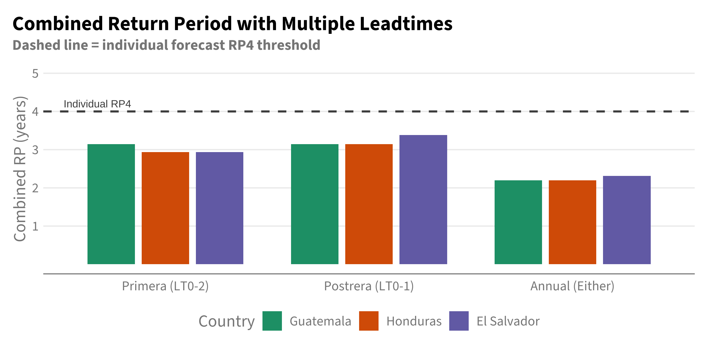
Combined return period vs individual forecast RP4. Using multiple leadtimes increases trigger frequency.

Key findings:

  • Primera combined RP ~2.5-3 years (vs RP4 individual) - using 3 leadtimes increases frequency
  • Postrera combined RP ~2.5-3 years - using 2 leadtimes has similar effect
  • Annual combined RP ~1.8-2.2 years - triggering in either season roughly doubles frequency vs single-season
  • Forecasts are correlated within-season, so combined RP is higher than theoretical independent assumption

Operational implication: With the recommended framework (Primera LT0-2, Postrera LT0-1), expect to trigger roughly every 2 years on average, not every 4 years. This is by design - multiple monitoring windows provide redundancy and earlier warning, but the cost is more frequent activations.

7.10.1 Threshold Tuning for Target Combined RP

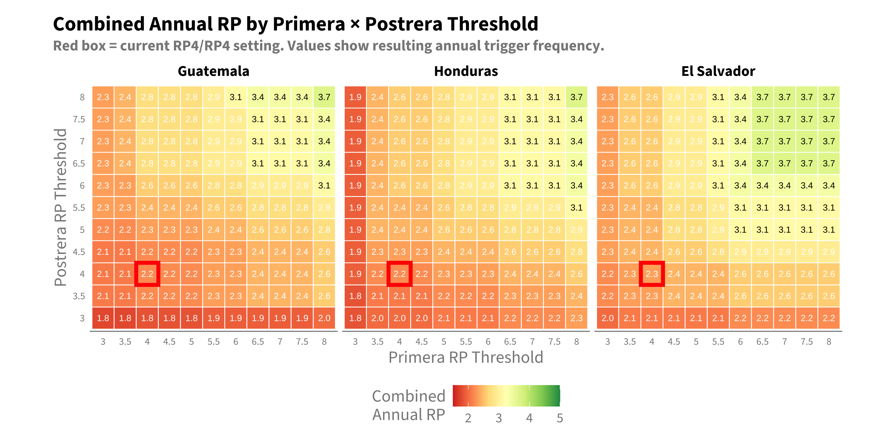
If a specific combined annual RP is desired (e.g., RP3 or RP4 annually), we can adjust the per-season thresholds. The heatmap below shows how different Primera and Postrera RP thresholds combine to produce a total annual RP.

Code
# Grid of RP thresholds to test
rp_grid <- seq(3, 8, by = 0.25)

# Function to calculate combined annual RP for given thresholds
calc_combined_rp <- function(df, primera_rp, postrera_rp, primera_lts = 0:2, postrera_lts = 0:1) {

 # Calculate thresholds for each RP level
  primera_thresh <- df |>
    filter(window == "primera", leadtime %in% primera_lts) |>
    group_by(country_aoi, leadtime) |>
    summarise(fcst_thresh = calc_rp_threshold(fcst_mm, primera_rp, -1), .groups = "drop")

  postrera_thresh <- df |>
    filter(window == "postrera", leadtime %in% postrera_lts) |>
    group_by(country_aoi, leadtime) |>
    summarise(fcst_thresh = calc_rp_threshold(fcst_mm, postrera_rp, -1), .groups = "drop")

  # Check triggers
  primera_triggers <- df |>
    filter(window == "primera", leadtime %in% primera_lts) |>
    left_join(primera_thresh, by = c("country_aoi", "leadtime")) |>
    mutate(triggered = fcst_mm <= fcst_thresh) |>
    group_by(country_aoi, year) |>
    summarise(primera_triggered = any(triggered), .groups = "drop")

  postrera_triggers <- df |>
    filter(window == "postrera", leadtime %in% postrera_lts) |>
    left_join(postrera_thresh, by = c("country_aoi", "leadtime")) |>
    mutate(triggered = fcst_mm <= fcst_thresh) |>
    group_by(country_aoi, year) |>
    summarise(postrera_triggered = any(triggered), .groups = "drop")

  # Combine and calculate annual RP
  primera_triggers |>
    left_join(postrera_triggers, by = c("country_aoi", "year")) |>
    mutate(annual_triggered = primera_triggered | postrera_triggered) |>
    group_by(country_aoi) |>
    summarise(
      trigger_rate = mean(annual_triggered, na.rm = TRUE),
      combined_rp = 1 / trigger_rate,
      .groups = "drop"
    )
}

# Calculate for all combinations
df_baseline <- df_joined |> filter(year >= 1981, year <= 2024)

df_rp_grid <- expand_grid(
  primera_rp = rp_grid,
  postrera_rp = rp_grid
) |>
  mutate(
    results = map2(primera_rp, postrera_rp, ~calc_combined_rp(df_baseline, .x, .y))
  ) |>
  unnest(results)
Code
# Use coarser grid with text labels for readability
df_rp_coarse <- df_rp_grid |>
  filter(primera_rp %in% seq(3, 8, by = 0.5), postrera_rp %in% seq(3, 8, by = 0.5)) |>
  mutate(
    country_aoi = factor(country_aoi, levels = c("Guatemala", "Honduras", "El Salvador")),
    rp_label = sprintf("%.1f", combined_rp),
    is_rp4 = primera_rp == 4 & postrera_rp == 4
  )

df_rp_coarse |>
  ggplot(aes(x = factor(primera_rp), y = factor(postrera_rp), fill = combined_rp)) +
  geom_tile(color = "white", linewidth = 0.3) +
  geom_text(aes(label = rp_label, color = combined_rp > 3), size = 2.5) +
  geom_tile(data = . %>% filter(is_rp4), fill = NA, color = "red", linewidth = 1.5) +
  facet_wrap(~country_aoi) +
  scale_fill_distiller(
    name = "Combined\nAnnual RP",
    palette = "RdYlGn",
    direction = 1,
    limits = c(1.5, 5),
    oob = scales::squish
  ) +
  scale_color_manual(values = c("TRUE" = "black", "FALSE" = "white"), guide = "none") +
  labs(
    title = "Combined Annual RP by Primera × Postrera Threshold",
    subtitle = "Red box = current RP4/RP4 setting. Values show resulting annual trigger frequency.",
    x = "Primera RP Threshold", y = "Postrera RP Threshold"
  ) +
  coord_fixed() +
  theme(
    strip.text = element_text(size = 12, face = "bold"),
    panel.grid = element_blank(),
    axis.text = element_text(size = 8)
  )

Combined annual RP as a function of Primera and Postrera thresholds.
Code
# Find combinations closest to target RPs
target_rps <- c(2.5, 3, 4)

df_targets <- df_rp_grid |>
  cross_join(tibble(target_rp = target_rps)) |>
  mutate(distance = abs(combined_rp - target_rp)) |>
  group_by(country_aoi, target_rp) |>
  slice_min(distance, n = 1, with_ties = FALSE) |>
  ungroup() |>
  mutate(
    setting = sprintf("P:RP%.1f / S:RP%.1f", primera_rp, postrera_rp),
    actual_rp = sprintf("%.2f yr", combined_rp)
  ) |>
  select(country_aoi, target_rp, setting, actual_rp) |>
  pivot_wider(
    names_from = target_rp,
    values_from = c(setting, actual_rp),
    names_glue = "RP{target_rp}_{.value}"
  )

df_targets |>
  gt() |>
  tab_header(
    title = md("**Threshold Settings for Target Annual RP**"),
    subtitle = "Primera (P) and Postrera (S) RP thresholds to achieve desired combined frequency"
  ) |>
  cols_label(
    country_aoi = "Country",
    `RP2.5_setting` = "Setting",
    `RP2.5_actual_rp` = "Actual",
    RP3_setting = "Setting",
    RP3_actual_rp = "Actual",
    RP4_setting = "Setting",
    RP4_actual_rp = "Actual"
  ) |>
  tab_spanner(label = md("**Target RP 2.5**"), columns = starts_with("RP2.5")) |>
  tab_spanner(label = md("**Target RP 3**"), columns = starts_with("RP3")) |>
  tab_spanner(label = md("**Target RP 4**"), columns = starts_with("RP4")) |>
  tab_footnote(
    footnote = "P = Primera threshold, S = Postrera (Postrera) threshold",
    locations = cells_column_labels(columns = `RP2.5_setting`)
  )
Threshold combinations to achieve target combined annual RP
Threshold Settings for Target Annual RP
Primera (P) and Postrera (S) RP thresholds to achieve desired combined frequency
Country Target RP 2.5 Target RP 3 Target RP 4
Setting1 Actual Setting Actual Setting Actual
El Salvador P:RP3.5 / S:RP4.2 2.44 yr P:RP4.2 / S:RP5.8 2.93 yr P:RP6.5 / S:RP6.5 3.67 yr
Guatemala P:RP3.2 / S:RP6.5 2.44 yr P:RP5.2 / S:RP6.5 2.93 yr P:RP7.8 / S:RP7.8 3.67 yr
Honduras P:RP3.5 / S:RP4.8 2.44 yr P:RP5.2 / S:RP5.8 2.93 yr P:RP7.8 / S:RP7.8 3.67 yr
1 P = Primera threshold, S = Postrera (Postrera) threshold

Reading the heatmap:

  • Bottom-left (low RP thresholds) = frequent triggers, low combined RP
  • Top-right (high RP thresholds) = rare triggers, high combined RP
  • The red X marks current RP4/RP4 setting
  • White contour lines show where combined annual RP equals 2, 3, 4, or 5 years

To achieve combined annual RP of ~4 years (triggering once every 4 years on average), you would need to set individual thresholds around RP5-6 for each season, depending on the country.

7.11 Recommendations

Based on this multi-AOI assessment:

  1. Use the 1981-2024 baseline for threshold calculation. The longer record provides more stable estimates and reveals skill that is masked by the shorter baseline.

  2. Primera forecasts are reliable across all three countries at LT0-2. Any of these leadtimes can be used operationally.

  3. Postrera: Use LT0 and LT1:

    • LT1 (August-issued): Primary forecast for preparedness planning (~1 month lead time, ROC-AUC 0.72-0.79)
    • LT0 (September-issued): Confirmation/update as season begins (ROC-AUC 0.80-0.87)
    • LT2-3 show weaker skill and are less reliable for operational decisions
  4. Regional considerations:

    • Honduras Postrera forecasts are most reliable across all leadtimes
    • Guatemala Postrera should be interpreted with more caution
    • El Salvador shows strong improvement with longer baseline
  5. For Guatemala specifically: Given the weaker Postrera skill, consider:

    • Emphasizing Primera forecasts for anticipatory action
    • Using Postrera forecasts as one input among several (ENSO state, VHI, etc.)
    • Relying primarily on LT0-1 for Postrera decisions