6 Leadtime Diagnostics

6.1 Motivation

In Chapter 4, CCSM4 showed a suspicious pattern for Postrera: skill at LT2-3 exceeded skill at LT1. This is backwards—forecast skill should degrade with increasing leadtime, not improve.

This chapter investigates whether this pattern reflects genuine predictability or a data quality issue by examining:

Inter-leadtime correlations: Do consecutive leadtimes agree with each other?
Coefficient of Variation (CV): Do forecasts show realistic interannual variability?

Setup

library(tidyverse)
library(lubridate)
library(cumulus)
library(gghdx)
gghdx()

box::use(../../R/enacts)
box::use(../../R/seas5)

BASELINE_START <- 2000
BASELINE_END <- 2024
PRIMERA_MONTHS <- 5:8
POSTRERA_MONTHS <- 9:11

Load forecast and observation data

# Forecasts
df_insiv <- cumulus::blob_read(
  name = "ds-aa-lac-dry-corridor/data/processed/insivumeh_special/insivumeh_special_models_zonal_seasonal_chiquimula.parquet",
  container = "projects"
)
df_seas5 <- seas5$load_seas5_seasonal()

# Observations
df_enacts <- enacts$load_enacts_seasonal("chiquimula")

# Combine forecasts
df_fcst_all <- bind_rows(df_insiv, df_seas5) |>
  filter(year >= BASELINE_START, year <= BASELINE_END) |>
  mutate(model = str_remove(forecast_source, "INSIVUMEH_"))

6.2 Inter-Leadtime Correlations

For a well-behaved forecast system, predictions at different leadtimes for the same target season should be correlated—they’re all trying to predict the same thing. If LT1 and LT2 forecasts are uncorrelated, one or both must be essentially random.

Function to compute correlation matrix

compute_lt_corr_matrix <- function(df, model_name, window_name) {
  df_wide <- df |>
    filter(model == model_name, window == window_name, !is.na(leadtime)) |>
    select(year, leadtime, value) |>
    pivot_wider(names_from = leadtime, values_from = value, names_prefix = "LT")

  # Add observations
  df_obs <- df_enacts |>
    filter(window == window_name, year >= BASELINE_START, year <= BASELINE_END) |>
    select(year, obs_mm)

  df_wide <- df_wide |>
    left_join(df_obs, by = "year") |>
    rename(OBS = obs_mm)

  # Compute correlation matrix - only keep LT and OBS columns
  cor_mat <- df_wide |>
    select(starts_with("LT"), OBS) |>
    cor(use = "pairwise.complete.obs")

  cor_mat
}

SEAS5 inter-leadtime correlations

models <- unique(df_fcst_all$model)
windows <- c("primera", "postrera")

# Compute all correlation matrices
corr_results <- expand_grid(model = models, window = windows) |>
  mutate(
    corr_mat = map2(model, window, ~compute_lt_corr_matrix(df_fcst_all, .x, .y))
  )

6.2.1 SEAS5 Correlation Patterns

Code

# Extract SEAS5 matrices
seas5_primera <- corr_results |>
  filter(model == "SEAS5", window == "primera") |>
  pull(corr_mat) |>
  pluck(1)

seas5_postrera <- corr_results |>
  filter(model == "SEAS5", window == "postrera") |>
  pull(corr_mat) |>
  pluck(1)

# Convert to long format for plotting (lower triangle only)
mat_to_df <- function(mat, label) {
  var_order <- c("LT4", "LT3", "LT2", "LT1", "OBS")
  # Filter to only include columns that exist in the matrix
  var_order <- var_order[var_order %in% colnames(mat)]

  as.data.frame(mat) |>
    mutate(row = rownames(mat)) |>
    pivot_longer(-row, names_to = "col", values_to = "cor") |>
    mutate(
      label = label,
      row_idx = match(row, var_order),
      col_idx = match(col, var_order)
    ) |>
    # Keep lower triangle only (row_idx > col_idx)
    filter(row_idx > col_idx) |>
    select(-row_idx, -col_idx)
}

df_seas5_corr <- bind_rows(
  mat_to_df(seas5_primera, "Primera"),
  mat_to_df(seas5_postrera, "Postrera")
) |> 
  mutate(
    label = fct_relevel(label, "Primera","Postrera")
  )

df_seas5_corr |>
  mutate(
    row = factor(row, levels = rev(c("LT4", "LT3", "LT2", "LT1", "OBS"))),
    col = factor(col, levels = c("LT4", "LT3", "LT2", "LT1", "OBS"))
  ) |>
  ggplot(aes(x = col, y = row, fill = cor)) +
  geom_tile(color = "white") +
  geom_text(aes(label = sprintf("%.2f", cor)), size = 3, fontface = "bold", color = "black") +
  facet_wrap(~label, scales = "free_x") +
  scale_fill_gradient2(low = "#D73027", mid = "white", high = "#1A9850", midpoint = 0.4, limits = c(-1, 1)) +
  labs(
    title = "SEAS5: Inter-Leadtime Correlations",
    subtitle = "Adjacent leadtimes should correlate strongly",
    x = NULL, y = NULL, fill = "Correlation",
    caption = "Omitting leadtime 0 as it is not available from INSVIUMEH provided models"
  ) +
  theme(legend.position = "right",plot.caption = element_text(hjust= 0,vjust=-1))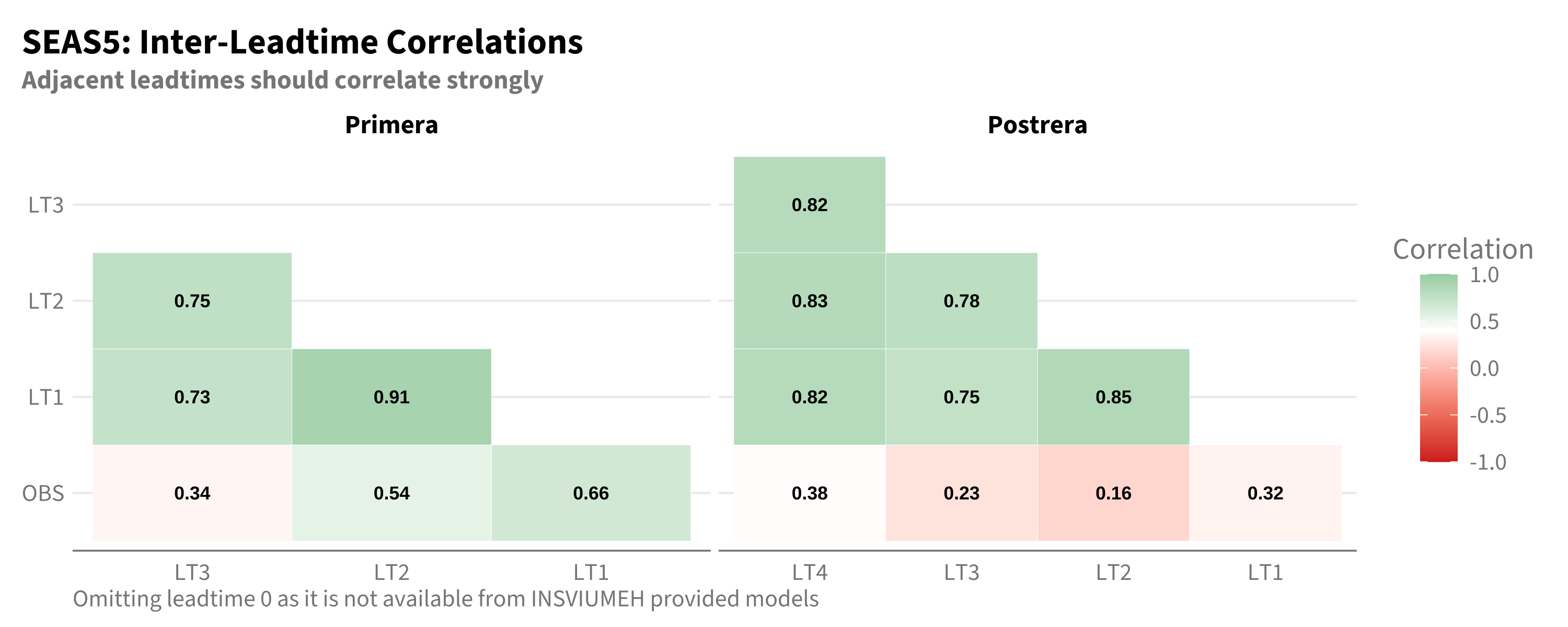

SEAS5 shows expected behavior: Adjacent leadtimes correlate at 0.6-0.9. LT1 correlates best with observations. This is a well-behaved forecast system.

6.2.2 INSIVUMEH Correlation Patterns

Code

# Extract INSIVUMEH matrices for all models
insiv_models <- c("CFSv2", "CCSM4", "CESM1")

df_insiv_corr <- map_dfr(insiv_models, function(m) {
  map_dfr(windows, function(w) {
    mat <- corr_results |>
      filter(model == m, window == w) |>
      pull(corr_mat) |>
      pluck(1)

    if (is.null(mat)) return(NULL)

    mat_to_df(mat, m) |>
      mutate(window = w)
  })
})

df_insiv_corr |>
  filter(!is.na(row), !is.na(col)) |>
  mutate(
    row = factor(row, levels = rev(c("LT4", "LT3", "LT2", "LT1", "OBS"))),
    col = factor(col, levels = c("LT4", "LT3", "LT2", "LT1", "OBS")),
    window = str_to_title(window),
    window = fct_relevel(window, "Primera","Postrera")
  ) |>
  ggplot(aes(x = col, y = row, fill = cor)) +
  geom_tile(color = "white") +
  geom_text(aes(label = sprintf("%.2f", cor)), size = 2.5, fontface = "bold", color = "black") +
  facet_grid(label ~ window, scales = "free_x") +
  scale_fill_gradient2(low = "#D73027", mid = "white", high = "#1A9850", midpoint = 0.4, limits = c(-1, 1)) +
  labs(
    title = "INSIVUMEH Models: Inter-Leadtime Correlations",
    subtitle = "Postrera shows near-zero or negative correlations between leadtimes",
    x = NULL, y = NULL, fill = "Correlation"
  ) +
  theme(legend.position = "right")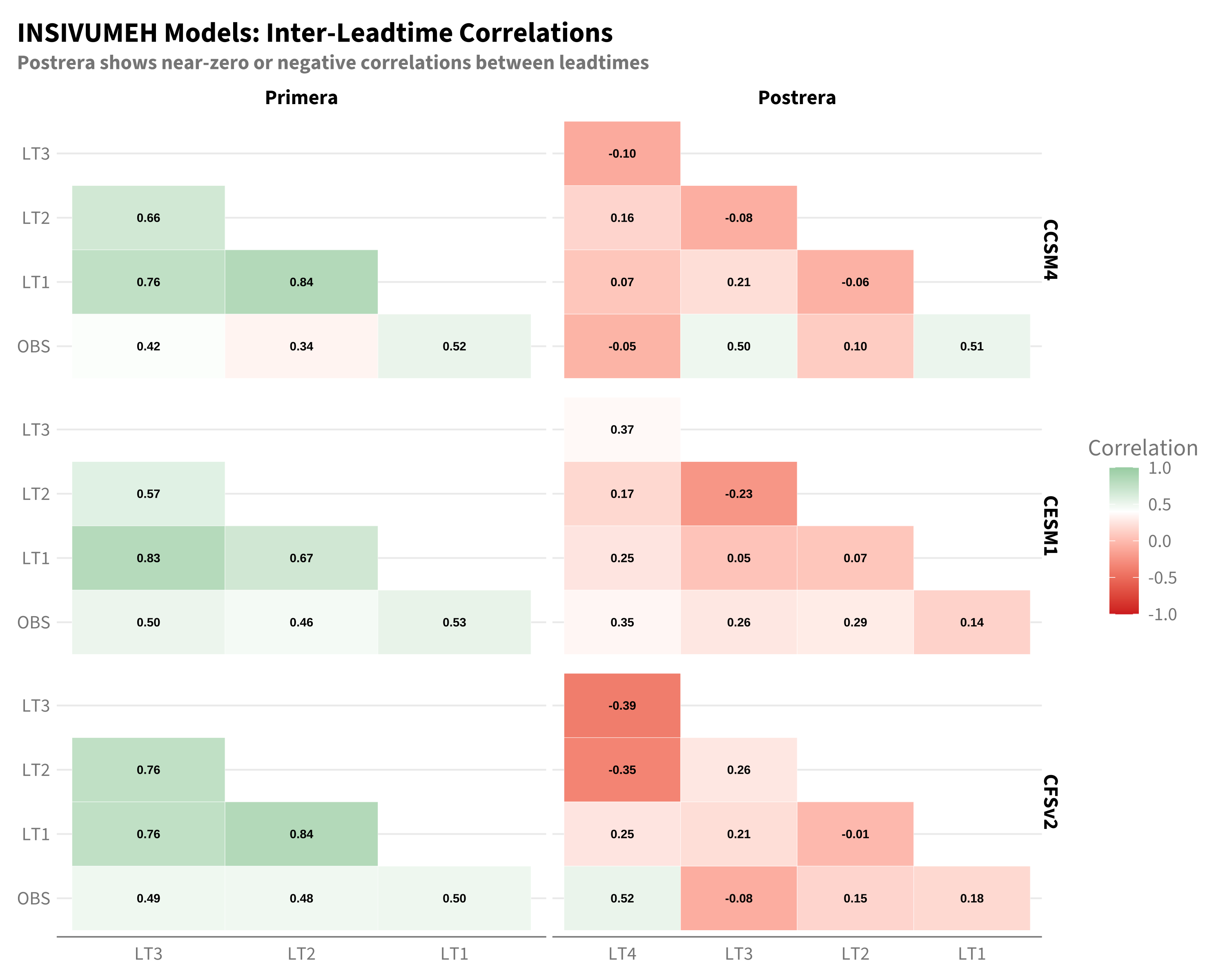

Critical finding: INSIVUMEH Postrera forecasts show near-zero or negative correlations between leadtimes. When LT1 predicts wet, LT2 might predict dry for the same target season. This is a fundamental data quality issue—these forecasts are not internally consistent.

6.3 Coefficient of Variation

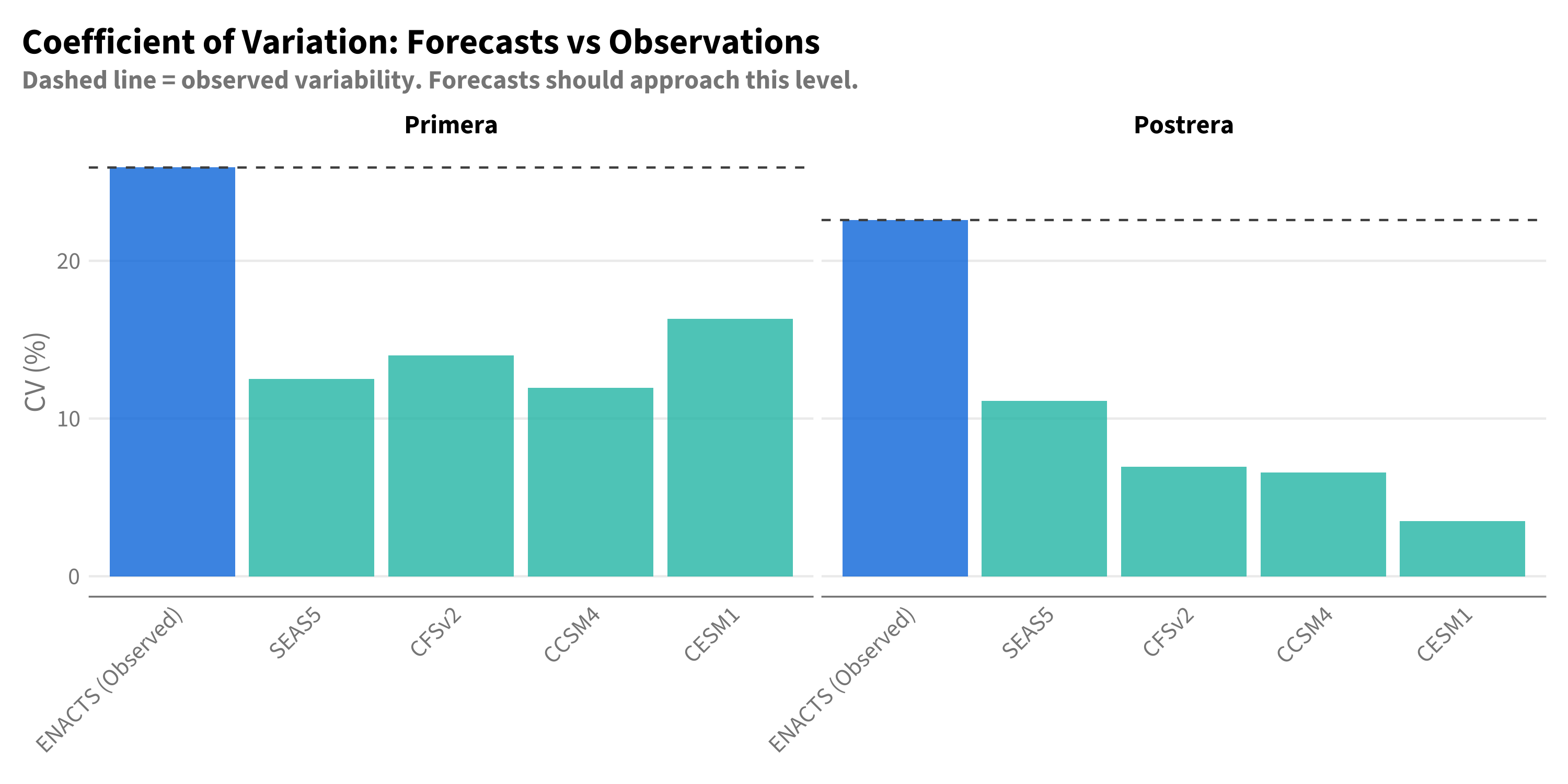
Another diagnostic: do forecasts show realistic interannual variability? A forecast that barely varies from year to year isn’t providing useful information, even if it occasionally correlates with observations.

Calculate CV for forecasts and observations

# Forecast CV
fcst_cv <- df_fcst_all |>
  filter(leadtime == 1) |>
  group_by(model, window) |>
  summarise(
    mean_mm = mean(value),
    sd_mm = sd(value),
    cv_pct = sd_mm / mean_mm * 100,
    .groups = "drop"
  )

# Observation CV
obs_cv <- df_enacts |>
  filter(year >= BASELINE_START, year <= BASELINE_END) |>
  group_by(window) |>
  summarise(
    mean_mm = mean(obs_mm),
    sd_mm = sd(obs_mm),
    cv_pct = sd_mm / mean_mm * 100,
    .groups = "drop"
  ) |>
  mutate(model = "ENACTS (Observed)")

# Combine
cv_all <- bind_rows(
  fcst_cv |> mutate(type = "Forecast"),
  obs_cv |> mutate(type = "Observed")
)

Code

cv_all |>
  mutate(
    model = factor(model, levels = c("ENACTS (Observed)", "SEAS5", "CFSv2", "CCSM4", "CESM1")),
    window = fct_relevel(str_to_title(window), "Primera", "Postrera")
  ) |>
  ggplot(aes(x = model, y = cv_pct, fill = type)) +
  geom_col(alpha = 0.8) +
  geom_hline(
    data = obs_cv |> mutate(window = fct_relevel(str_to_title(window), "Primera", "Postrera")),
    aes(yintercept = cv_pct),
    linetype = "dashed", color = "grey30"
  ) +
  facet_wrap(~window) +
  labs(
    title = "Coefficient of Variation: Forecasts vs Observations",
    subtitle = "Dashed line = observed variability. Forecasts should approach this level.",
    x = NULL, y = "CV (%)", fill = NULL
  ) +
  theme(
    axis.text.x = element_text(angle = 45, hjust = 1, vjust = 1),
    legend.position = "none"
  )

Code

cv_all |>
  select(model, window, cv_pct) |>
  mutate(window = str_to_title(window)) |>
  pivot_wider(names_from = window, values_from = cv_pct) |>
  select(model, Primera, Postrera) |>
  mutate(across(where(is.numeric), ~sprintf("%.1f%%", .x))) |>
  knitr::kable(caption = "Coefficient of Variation by Model and Season")

Coefficient of Variation by Model and Season
model	Primera	Postrera
CCSM4	11.9%	6.6%
CESM1	16.3%	3.5%
CFSv2	14.0%	6.9%
SEAS5	12.5%	11.1%
ENACTS (Observed)	25.9%	22.6%

Key findings (shown here for LT1 for simplicity):

Observed CV: Primera ~14%, Postrera ~23%
SEAS5: Reasonable CV for both seasons (8-15%), approaching observed variability
INSIVUMEH Primera: Moderate CV (10-18%), usable signal
INSIVUMEH Postrera: Very low CV (3-7%), forecasts barely vary from climatology

This pattern holds across all leadtimes—see the expanded analysis in the collapsible section below.

Robustness Check: CV Across Leadtimes and Observation Sources

Does the low CV pattern for INSIVUMEH Postrera hold across all leadtimes? And how does it compare to multiple observation sources?

Load additional observation sources and calculate CV across leadtimes

# Forecast CV across all leadtimes
fcst_cv_all_lt <- df_fcst_all |>
  group_by(model, window, leadtime) |>
  summarise(
    mean_mm = mean(value),
    sd_mm = sd(value),
    cv_pct = sd_mm / mean_mm * 100,
    .groups = "drop"
  )

# Load ERA5
con <- pg_con()
df_era5_raw <- tbl(con, "era5") |>
  filter(pcode == "GT20") |>
  collect() |>
  mutate(
    year = year(valid_date),
    month = month(valid_date),
    mean = mean * days_in_month(valid_date)
  )
DBI::dbDisconnect(con)

df_era5 <- bind_rows(
  df_era5_raw |>
    filter(month %in% PRIMERA_MONTHS) |>
    group_by(year) |>
    summarise(obs_mm = sum(mean), .groups = "drop") |>
    mutate(window = "primera"),
  df_era5_raw |>
    filter(month %in% POSTRERA_MONTHS) |>
    group_by(year) |>
    summarise(obs_mm = sum(mean), .groups = "drop") |>
    mutate(window = "postrera")
) |>
  filter(year >= BASELINE_START, year <= BASELINE_END)

# Load CHIRPS
df_chirps_raw <- cumulus::blob_read(
  name = "ds-aa-lac-dry-corridor/raw/chirps/2026_cadc_drought_v3_aoi_chirps_monthly_historical.parquet",
  container = "projects"
)

df_chirps <- df_chirps_raw |>
  filter(ADM1_NAME == "Chiquimula") |>
  mutate(
    year = year(date),
    month = month(date),
    window = case_when(
      month %in% PRIMERA_MONTHS ~ "primera",
      month %in% POSTRERA_MONTHS ~ "postrera",
      TRUE ~ NA_character_
    )
  ) |>
  filter(!is.na(window), year >= BASELINE_START, year <= BASELINE_END) |>
  group_by(year, window) |>
  summarise(obs_mm = sum(value, na.rm = TRUE), .groups = "drop")

# Calculate observed CV from all three sources
obs_cv_all <- bind_rows(
  df_enacts |>
    filter(year >= BASELINE_START, year <= BASELINE_END) |>
    group_by(window) |>
    summarise(cv_pct = sd(obs_mm) / mean(obs_mm) * 100, .groups = "drop") |>
    mutate(source = "ENACTS"),
  df_era5 |>
    group_by(window) |>
    summarise(cv_pct = sd(obs_mm) / mean(obs_mm) * 100, .groups = "drop") |>
    mutate(source = "ERA5"),
  df_chirps |>
    group_by(window) |>
    summarise(cv_pct = sd(obs_mm) / mean(obs_mm) * 100, .groups = "drop") |>
    mutate(source = "CHIRPS")
)

Create color-coded CV table

library(gt)

# Get observed CV range for reference
obs_cv_summary <- obs_cv_all |>
  group_by(window) |>
  summarise(
    obs_mean = mean(cv_pct),
    obs_min = min(cv_pct),
    obs_max = max(cv_pct),
    .groups = "drop"
  )

# Create wide table for gt
df_cv_wide <- fcst_cv_all_lt |>
  mutate(
    col_name = paste0(str_to_title(window), " LT", leadtime)
  ) |>
  select(model, col_name, cv_pct) |>
  pivot_wider(names_from = col_name, values_from = cv_pct)

# Add observed row (using mean across sources)
obs_row <- obs_cv_all |>
  group_by(window) |>
  summarise(cv_pct = mean(cv_pct), .groups = "drop") |>
  mutate(col_name = paste0(str_to_title(window), " (Obs)")) |>
  pivot_wider(names_from = col_name, values_from = cv_pct) |>
  mutate(model = "Observed (mean)")

# Combine and order
df_cv_wide <- df_cv_wide |>
  mutate(model = factor(model, levels = c("SEAS5", "CFSv2", "CCSM4", "CESM1"))) |>
  arrange(model) |>
  mutate(model = as.character(model))

# Define column order
primera_cols <- paste0("Primera LT", 1:3)
postrera_cols <- paste0("Postrera LT", 1:3)
all_cols <- c(primera_cols, postrera_cols)
all_cols <- all_cols[all_cols %in% names(df_cv_wide)]

df_cv_wide |>
  select(model, all_of(all_cols)) |>
  gt(rowname_col = "model") |>
  tab_header(
    title = "Coefficient of Variation by Model, Season, and Leadtime",
    subtitle = "Higher CV = more interannual variability (closer to observations)"
  ) |>
  tab_spanner(label = "Primera", columns = starts_with("Primera")) |>
  tab_spanner(label = "Postrera", columns = starts_with("Postrera")) |>
  fmt_number(columns = everything(), decimals = 1, pattern = "{x}%") |>
  data_color(
    columns = starts_with("Primera"),
    palette = c("#D73027", "#FFFFBF", "#1A9850"),
    domain = c(0, obs_cv_summary |> filter(window == "primera") |> pull(obs_mean))
  ) |>
  data_color(
    columns = starts_with("Postrera"),
    palette = c("#D73027", "#FFFFBF", "#1A9850"),
    domain = c(0, obs_cv_summary |> filter(window == "postrera") |> pull(obs_mean))
  ) |>
  tab_source_note(
    source_note = sprintf(
      "Observed CV: Primera %.0f-%.0f%%, Postrera %.0f-%.0f%% (across ENACTS, ERA5, CHIRPS)",
      obs_cv_summary |> filter(window == "primera") |> pull(obs_min),
      obs_cv_summary |> filter(window == "primera") |> pull(obs_max),
      obs_cv_summary |> filter(window == "postrera") |> pull(obs_min),
      obs_cv_summary |> filter(window == "postrera") |> pull(obs_max)
    )
  ) |>
  tab_style(
    style = cell_text(weight = "bold"),
    locations = cells_stub()
  ) |>
  cols_label_with(fn = ~str_remove(.x, "Primera |Postrera "))

	Primera			Postrera
Coefficient of Variation by Model, Season, and Leadtime
Higher CV = more interannual variability (closer to observations)
	LT1	LT2	LT3	LT1	LT2	LT3
SEAS5	12.5%	11.8%	10.5%	11.1%	11.2%	11.5%
CFSv2	14.0%	11.5%	10.7%	6.9%	5.1%	6.1%
CCSM4	11.9%	12.2%	10.1%	6.6%	6.8%	9.0%
CESM1	16.3%	11.7%	12.3%	3.5%	3.2%	6.3%
Observed CV: Primera 18-26%, Postrera 22-34% (across ENACTS, ERA5, CHIRPS)

Code

# Postrera-only bar plot with labeled observation lines
obs_cv_postrera <- obs_cv_all |>
  filter(window == "postrera") |>
  mutate(label_x = 3.5)  # Position for labels

fcst_cv_all_lt |>
  filter(window == "postrera") |>
  ggplot(aes(x = factor(leadtime), y = cv_pct, fill = model)) +
  geom_col(position = "dodge", alpha = 0.8) +
  geom_hline(
    data = obs_cv_postrera,
    aes(yintercept = cv_pct, linetype = source),
    inherit.aes = FALSE,
    color = "grey30"
  ) +
  geom_text(
    data = obs_cv_postrera,
    aes(x = label_x, y = cv_pct, label = source),
    inherit.aes = FALSE,
    hjust = 0, vjust = -0.3, size = 3, color = "grey30"
  ) +
  scale_linetype_manual(values = c("ENACTS" = "dashed", "ERA5" = "dotted", "CHIRPS" = "longdash")) +
  coord_cartesian(xlim = c(0.5, 4.2), clip = "off") +
  labs(
    title = "Postrera: Forecast CV vs Observed Variability",
    subtitle = "INSIVUMEH models show almost no interannual variation",
    x = "Leadtime", y = "CV (%)", fill = "Model"
  ) +
  theme(legend.position = "bottom") +
  guides(linetype = "none")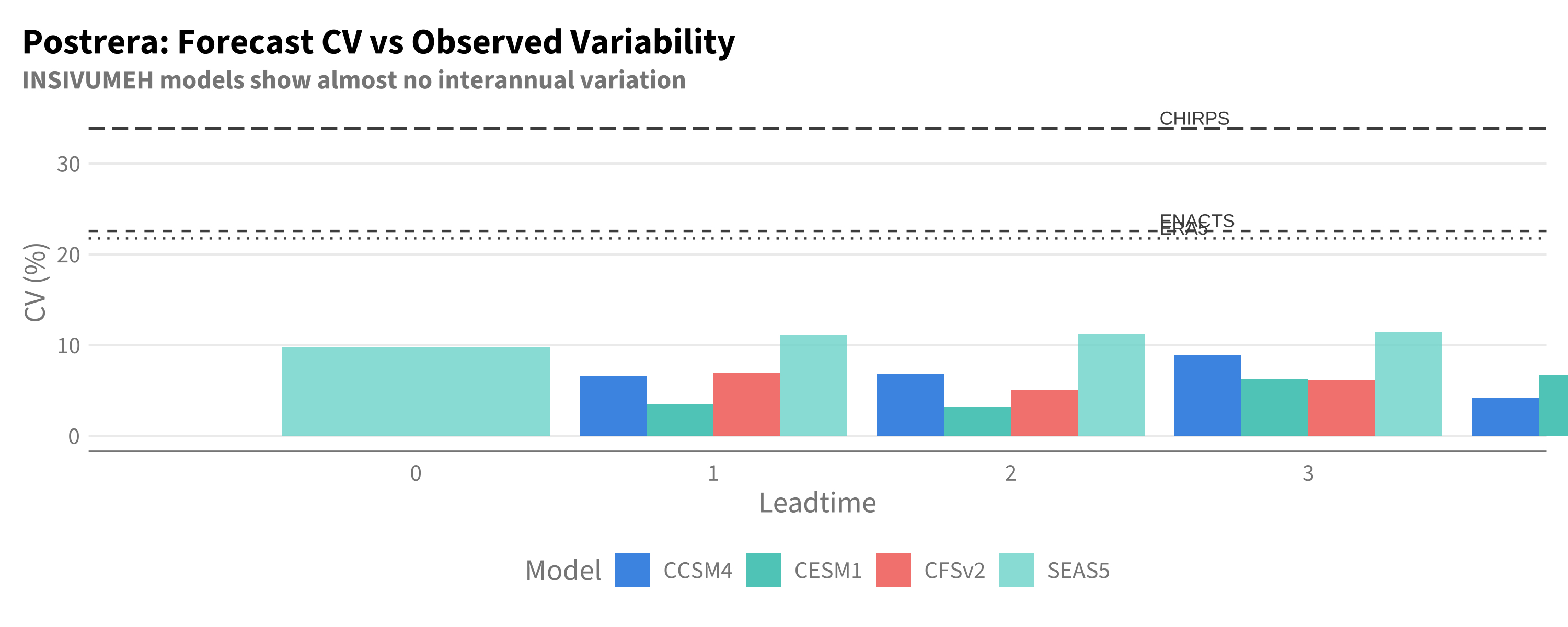

The pattern holds: INSIVUMEH Postrera CV remains very low (3-7%) across all leadtimes, far below observed variability from any source. This is not a leadtime-specific issue—the Postrera forecasts systematically lack interannual signal.

6.4 Implications

The diagnostic tests reveal a fundamental issue with INSIVUMEH Postrera forecasts:

Diagnostic	SEAS5	INSIVUMEH Primera	INSIVUMEH Postrera
Inter-LT correlation	High (0.6-0.9)	Moderate (0.3-0.7)	Near-zero or negative
CV vs observed	~70% of observed	~80% of observed	~20% of observed
Signal strength	Strong	Moderate	Limited

This explains the suspicious patterns in Chapter 4:

Why CCSM4 LT3 > LT1 for Postrera: If leadtimes are uncorrelated, apparent “skill” at any leadtime is random. By chance, LT3 happened to correlate better with observations than LT1 in this sample.
Why INSIVUMEH Postrera shows erratic skill: The forecasts contain almost no signal—they’re essentially flat lines near climatology with random noise.
Why skill scores are unreliable: When forecasts don’t vary, correlations are dominated by noise and small-sample coincidences.

6.5 The Real Tie-Breaker for Postrera

The skill metrics in earlier chapters were inconclusive for Postrera—no model showed consistent skill, and the patterns were erratic. These diagnostics break the tie.

The issue isn’t that INSIVUMEH Postrera forecasts lack skill—it’s that they lack signal. A forecast that barely varies from climatology and shows no internal consistency between leadtimes cannot be operationally useful, regardless of what correlation metrics suggest.

Postrera recommendation: SEAS5

Not because SEAS5 has demonstrated strong Postrera skill (it hasn’t), but because:

SEAS5 is internally consistent—different leadtimes agree with each other
SEAS5 shows realistic interannual variability
SEAS5 at least behaves like a forecast, even if predictability is limited

INSIVUMEH Postrera forecasts show limited predictive signal for this region and season.

6.6 Final Recommendations

Season	Recommended	Rationale
Primera	SEAS5	Clear skill advantage across metrics and observation sources
Postrera	SEAS5	INSIVUMEH forecasts show limited signal (low CV, weak inter-leadtime consistency)

For Postrera specifically, consider:

Acknowledging limited predictability in operational communications
Using shorter-range forecasts when available
Supplementing forecast-based triggers with monitoring-based indicators (e.g., observed rainfall deficits or VHI during early Postrera)