8  AOI Sensitivity Exploration

8.1 Overview

Chapter 07 established SEAS5 skill using the original framework AOI:

• Guatemala: Chiquimula (GT20)
• Honduras: El Paraíso + Francisco Morazán (HN07/HN08).
• El Salvador: Ahuachapán + Santa Ana (SV01/SV12)

This chapter explores two dimensions of geographic sensitivity:

1. Admin expansion: Does adding neighbouring admin units (GT16 Zacapa, SV13 Morazán, SV05 La Libertad) change skill?
2. Spatial scale: How does country-level aggregation compare to sub-national?

8.2 Data Preparation

PRIMERA_MONTHS <- 5:8
POSTRERA_MONTHS <- 9:11
PRIMERA_ISSUED_MONTHS <- c(3, 4, 5)
POSTRERA_ISSUED_MONTHS <- c(6, 7, 8, 9)

# All candidate admin-1 pcodes
CANDIDATE_PCODES <- c(
  "GT20", "GT16",          # Guatemala: Chiquimula, Alta Verapaz
  "GT19", "GT02",           # Guatemala: Zacapa, El Progreso
  "GT21",                  # Guatemala: Jalapa
  "GT14", "GT15",          # Guatemala: Quiché, Baja Verapaz
  "HN07", "HN08",          # Honduras: El Paraíso, Francisco Morazán
  "SV01", "SV12",          # El Salvador confirmed: Ahuachapán, Santa Ana
  "SV13", "SV05"           # El Salvador candidates: Morazán, La Libertad
)

con <- pg_con()

df_weights <- tbl(con, "polygon") |>
  mutate(across(pcode, as.character)) |>
  filter(adm_level == 1, pcode %in% CANDIDATE_PCODES) |>
  select(pcode, iso3, name, seas5_n_upsampled_pixels) |>
  collect()

# Admin-1 level data
df_seas5_raw <- tbl(con, "seas5") |>
  mutate(across(pcode, as.character)) |>
  filter(adm_level == 1, pcode %in% CANDIDATE_PCODES) |>
  collect()

df_era5_raw <- tbl(con, "era5") |>
  mutate(across(pcode, as.character)) |>
  filter(pcode %in% CANDIDATE_PCODES) |>
  collect()

# Country-level (adm0) data
df_seas5_country <- tbl(con, "seas5") |>
  mutate(across(pcode, as.character)) |>
  filter(adm_level == 0, iso3 %in% c("GTM", "HND", "SLV")) |>
  collect()

df_era5_country <- tbl(con, "era5") |>
  mutate(across(pcode, as.character)) |>
  filter(adm_level == 0, iso3 %in% c("GTM", "HND", "SLV")) |>
  collect()

DBI::dbDisconnect(con)

# Process admin-1 to seasonal totals
df_seas5_mm <- df_seas5_raw |>
  mutate(value_mm = days_in_month(valid_date) * mean)

df_seas5_seasonal <- bind_rows(
  seas5_aggregate_forecast(df_seas5_mm, value = "value_mm", valid_months = PRIMERA_MONTHS,
                           by = c("iso3", "pcode", "issued_date")) |> mutate(window = "primera"),
  seas5_aggregate_forecast(df_seas5_mm, value = "value_mm", valid_months = POSTRERA_MONTHS,
                           by = c("iso3", "pcode", "issued_date")) |> mutate(window = "postrera")
) |>
  rename(fcst_mm = value_mm) |>
  mutate(
    year = year(issued_date),
    issued_month = month(issued_date)
  ) |>
  filter(
    (window == "primera" & issued_month %in% PRIMERA_ISSUED_MONTHS) |
    (window == "postrera" & issued_month %in% POSTRERA_ISSUED_MONTHS)
  )

df_era5_monthly <- df_era5_raw |>
  mutate(
    year = year(valid_date),
    month = month(valid_date),
    value_mm = mean * days_in_month(valid_date)
  )

df_era5_seasonal <- bind_rows(
  df_era5_monthly |>
    filter(month %in% PRIMERA_MONTHS) |>
    group_by(pcode, iso3, year) |>
    summarise(obs_mm = sum(value_mm), .groups = "drop") |>
    mutate(window = "primera"),
  df_era5_monthly |>
    filter(month %in% POSTRERA_MONTHS) |>
    group_by(pcode, iso3, year) |>
    summarise(obs_mm = sum(value_mm), .groups = "drop") |>
    mutate(window = "postrera")
)

# Process country-level to seasonal totals
df_seas5_country_mm <- df_seas5_country |>
  mutate(value_mm = days_in_month(valid_date) * mean)

df_seas5_country_seasonal <- bind_rows(
  seas5_aggregate_forecast(df_seas5_country_mm, value = "value_mm", valid_months = PRIMERA_MONTHS,
                           by = c("iso3", "pcode", "issued_date")) |> mutate(window = "primera"),
  seas5_aggregate_forecast(df_seas5_country_mm, value = "value_mm", valid_months = POSTRERA_MONTHS,
                           by = c("iso3", "pcode", "issued_date")) |> mutate(window = "postrera")
) |>
  rename(fcst_mm = value_mm) |>
  mutate(
    year = year(issued_date),
    issued_month = month(issued_date)
  ) |>
  filter(
    (window == "primera" & issued_month %in% PRIMERA_ISSUED_MONTHS) |
    (window == "postrera" & issued_month %in% POSTRERA_ISSUED_MONTHS)
  )

df_era5_country_monthly <- df_era5_country |>
  mutate(
    year = year(valid_date),
    month = month(valid_date),
    value_mm = mean * days_in_month(valid_date)
  )

df_era5_country_seasonal <- bind_rows(
  df_era5_country_monthly |>
    filter(month %in% PRIMERA_MONTHS) |>
    group_by(pcode, iso3, year) |>
    summarise(obs_mm = sum(value_mm), .groups = "drop") |>
    mutate(window = "primera"),
  df_era5_country_monthly |>
    filter(month %in% POSTRERA_MONTHS) |>
    group_by(pcode, iso3, year) |>
    summarise(obs_mm = sum(value_mm), .groups = "drop") |>
    mutate(window = "postrera")
)

calc_rp_threshold <- function(x, rp_target = 4, direction = -1) {
  x <- x[!is.na(x)]
  n <- length(x)
  if (n < 3) return(NA_real_)
  ranks <- rank(x * -direction, ties.method = "average")
  rp <- (n + 1) / ranks
  approx(rp, x, xout = rp_target, rule = 2)$y
}

calc_skill_metrics <- function(df, baseline_start = 1981, baseline_end = 2024, rp_target = 4) {
  df_baseline <- df |>
    filter(year >= baseline_start, year <= baseline_end)

  obs_thresholds <- df_baseline |>
    group_by(aoi_config, window) |>
    summarise(obs_thresh = calc_rp_threshold(obs_mm, rp_target, -1), .groups = "drop")

  fcst_thresholds <- df_baseline |>
    group_by(aoi_config, window, leadtime) |>
    summarise(fcst_thresh = calc_rp_threshold(fcst_mm, rp_target, -1), .groups = "drop")

  drought_levels <- c("drought", "no_drought")

  df_baseline |>
    left_join(obs_thresholds, by = c("aoi_config", "window")) |>
    left_join(fcst_thresholds, by = c("aoi_config", "window", "leadtime")) |>
    mutate(
      truth = fct(
        if_else(obs_mm <= obs_thresh, "drought", "no_drought"),
        levels = drought_levels
      ),
      estimate = fct(
        if_else(fcst_mm <= fcst_thresh, "drought", "no_drought"),
        levels = drought_levels
      )
    ) |>
    filter(!is.na(truth), !is.na(estimate)) |>
    group_by(aoi_config, window, leadtime) |>
    summarise(
      n_years = n_distinct(year),
      n_drought = sum(truth == "drought"),
      spearman = cor(fcst_mm, obs_mm, method = "spearman", use = "complete.obs"),
      roc_auc = roc_auc_vec(truth, -fcst_mm, event_level = "first"),
      f1 = f_meas_vec(truth, estimate, event_level = "first"),
      .groups = "drop"
    )
}

8.3 Rainfall Coherence Map

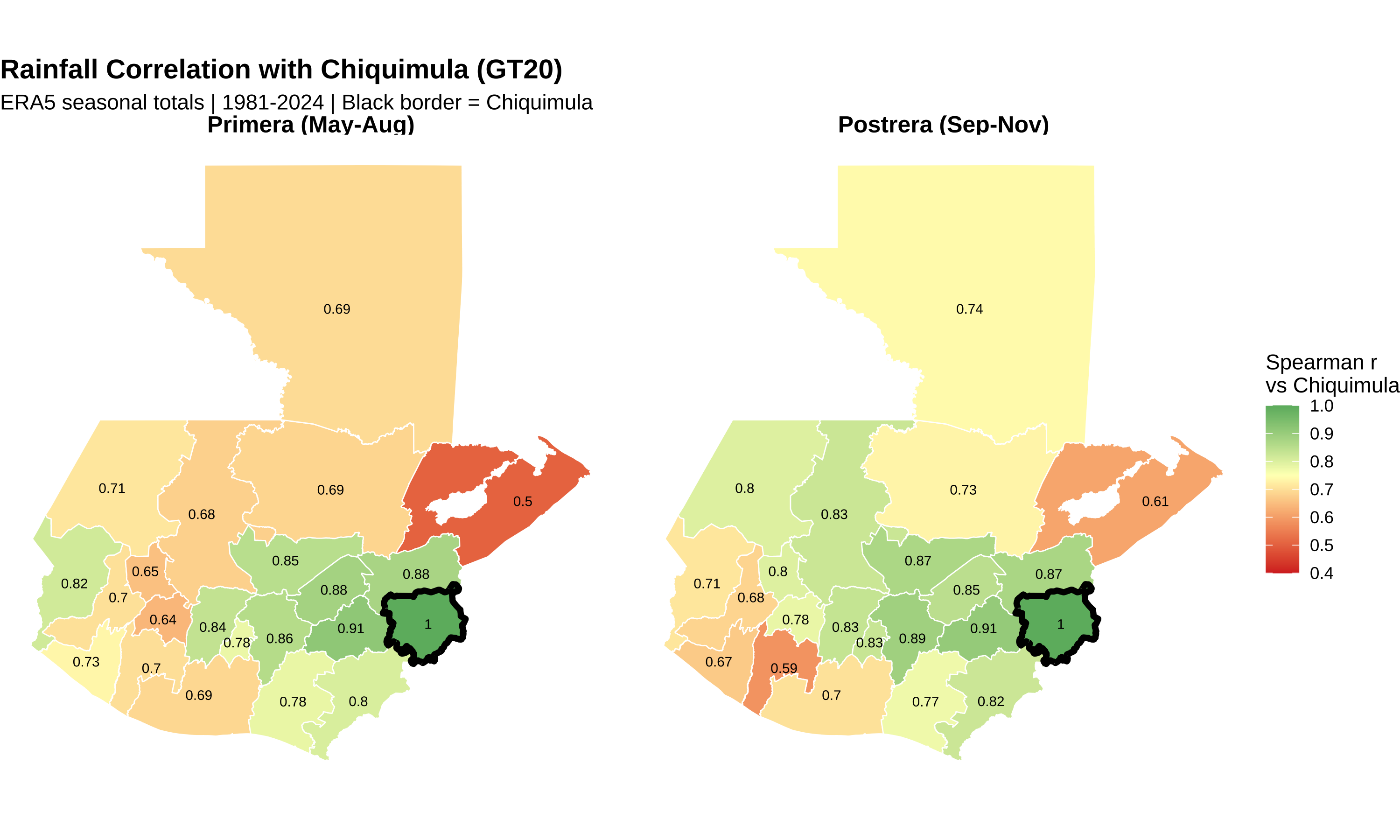
Before examining forecast skill across AOI configurations, we first check how well seasonal rainfall in each Guatemala department correlates with Chiquimula (GT20) — the current framework AOI. Departments with low correlation experience droughts at different times, making them poor candidates for combining into a single trigger.

# Get all GTM admin-1 ERA5 data
con <- pg_con()

df_era5_gtm_all <- tbl(con, "era5") |>
  mutate(across(pcode, as.character)) |>
  filter(iso3 == "GTM", adm_level == 1) |>
  collect()

DBI::dbDisconnect(con)

# Get admin-1 boundaries
gdf_gtm <- cumulus::download_fieldmaps_sf(iso3 = "gtm", layer = "gtm_adm1")$gtm_adm1

# Aggregate to seasonal totals
df_gtm_monthly <- df_era5_gtm_all |>
  mutate(
    year = year(valid_date),
    month = month(valid_date),
    value_mm = mean * days_in_month(valid_date)
  )

df_gtm_seasonal <- bind_rows(
  df_gtm_monthly |>
    filter(month %in% PRIMERA_MONTHS) |>
    group_by(pcode, year) |>
    summarise(obs_mm = sum(value_mm), .groups = "drop") |>
    mutate(window = "primera"),
  df_gtm_monthly |>
    filter(month %in% POSTRERA_MONTHS) |>
    group_by(pcode, year) |>
    summarise(obs_mm = sum(value_mm), .groups = "drop") |>
    mutate(window = "postrera")
) |>
  filter(year >= 1981)

# Calculate Spearman correlation of each admin with GT20
gt20_obs <- df_gtm_seasonal |>
  filter(pcode == "GT20") |>
  select(year, window, obs_mm_gt20 = obs_mm)

df_cor_gt20 <- df_gtm_seasonal |>
  left_join(gt20_obs, by = c("year", "window")) |>
  group_by(pcode, window) |>
  summarise(
    spearman = cor(obs_mm, obs_mm_gt20, method = "spearman", use = "complete.obs"),
    .groups = "drop"
  )

# Join correlation to spatial data
# Match on pcode - fieldmaps may use different column name
pcode_col <- intersect(c("ADM1_PCODE", "adm1_pcode", "pcode"), names(gdf_gtm))[1]
gdf_gtm_cor <- gdf_gtm |>
  rename(pcode = !!pcode_col) |>
  left_join(df_cor_gt20, by = "pcode")

gdf_gtm_cor |>
  mutate(
    window_label = factor(window,
      levels = c("primera", "postrera"),
      labels = c("Primera (May-Aug)", "Postrera (Sep-Nov)")
    )
  ) |>
  ggplot() +
  geom_sf(aes(fill = spearman), color = "white", linewidth = 0.3) +
  geom_sf(
    data = gdf_gtm_cor |> filter(pcode == "GT20") |> head(1),
    fill = NA, color = "black", linewidth = 1.5
  ) +
  geom_sf_text(aes(label = round(spearman, 2)), size = 2.5, color = "black") +
  facet_wrap(~window_label) +
  scale_fill_gradient2(
    low = "#D73027", mid = "#FFFFBF", high = "#1A9850",
    midpoint = 0.75, limits = c(0.4, 1), name = "Spearman r\nvs Chiquimula",
    oob = scales::squish
  ) +
  labs(
    title = "Rainfall Correlation with Chiquimula (GT20)",
    subtitle = "ERA5 seasonal totals | 1981-2024 | Black border = Chiquimula"
  ) +
  theme_void() +
  theme(
    strip.text = element_text(size = 12, face = "bold"),
    legend.position = "right",
    plot.title = element_text(size = 14, face = "bold")
  )

8.4 Admin Expansion

How does skill change when we expand the geographic footprint within each country?

# Build pcode-to-name lookup from polygon table (all admin-1, not just those with SEAS5 data)
df_admin_names <- tbl(pg_con(), "polygon") |>
  mutate(across(pcode, as.character)) |>
  filter(adm_level == 1, pcode %in% CANDIDATE_PCODES) |>
  select(pcode, name) |>
  collect()
pcode_to_name <- setNames(df_admin_names$name, df_admin_names$pcode)

relabel_config <- function(config_name) {
  # "GTM: GT20+GT16" → "GTM: Chiquimula + Alta Verapaz"
  parts <- str_split(config_name, ": ", n = 2)[[1]]
  prefix <- parts[1]
  pcodes <- str_split(parts[2], "\\+")[[1]]
  names <- ifelse(pcodes %in% names(pcode_to_name), pcode_to_name[pcodes], pcodes)
  paste0(prefix, ": ", paste(names, collapse = " + "))
}

# Define AOI configurations to compare
aoi_configs <- list(
  # Guatemala
  "GTM: GT20" = c("GT20"),
  "GTM: GT20+GT16" = c("GT20", "GT16"),
  "GTM: GT20+GT19" = c("GT20", "GT19"),
  "GTM: GT20+GT02" = c("GT20", "GT02"),
  "GTM: GT20+GT21+GT02+GT19" = c("GT20", "GT21", "GT02", "GT19"),
  "GTM: GT20+GT21+GT02" = c("GT20", "GT21", "GT02"),
  "GTM: GT16" = c("GT16"),
  "GTM: GT15" = c("GT15"),
  "GTM: GT14" = c("GT14"),
  "GTM: GT14+GT15" = c("GT14", "GT15"),
  # Honduras
  "HND: HN07+HN08" = c("HN07", "HN08"),
  # El Salvador
  "SLV: SV01+SV12" = c("SV01", "SV12"),
  "SLV: SV01+SV12+SV13" = c("SV01", "SV12", "SV13"),
  "SLV: SV01+SV12+SV13+SV05" = c("SV01", "SV12", "SV13", "SV05")
)

# Relabel config names to use admin names
names(aoi_configs) <- map_chr(names(aoi_configs), relabel_config)

# Build weighted-mean aggregated datasets for each config
aggregate_config <- function(pcodes, config_name) {
  df_fcst <- df_seas5_seasonal |>
    filter(pcode %in% pcodes) |>
    left_join(df_weights |> select(pcode, seas5_n_upsampled_pixels), by = "pcode")

  df_obs <- df_era5_seasonal |>
    filter(pcode %in% pcodes) |>
    left_join(df_weights |> select(pcode, seas5_n_upsampled_pixels), by = "pcode")

  df_joined <- df_fcst |>
    left_join(
      df_obs |> select(pcode, year, window, obs_mm),
      by = c("pcode", "year", "window")
    ) |>
    filter(!is.na(obs_mm)) |>
    group_by(year, window, leadtime, issued_date) |>
    summarise(
      fcst_mm = weighted.mean(fcst_mm, w = seas5_n_upsampled_pixels),
      obs_mm = weighted.mean(obs_mm, w = seas5_n_upsampled_pixels),
      .groups = "drop"
    ) |>
    mutate(aoi_config = config_name)

  df_joined
}

df_all_configs <- imap_dfr(aoi_configs, ~aggregate_config(.x, .y))

# Add country-level configs
df_country_joined <- df_seas5_country_seasonal |>
  left_join(
    df_era5_country_seasonal |> select(pcode, year, window, obs_mm),
    by = c("pcode", "year", "window")
  ) |>
  filter(!is.na(obs_mm)) |>
  mutate(
    aoi_config = case_when(
      iso3 == "GTM" ~ "GTM: Country",
      iso3 == "HND" ~ "HND: Country",
      iso3 == "SLV" ~ "SLV: Country"
    )
  )

df_all_configs <- bind_rows(df_all_configs, df_country_joined)

df_skill_admin <- calc_skill_metrics(df_all_configs)

# Shared theme for faceted horizontal bar charts
theme_facet_bars <- theme(
  legend.position = "none",
  panel.spacing = unit(0.8, "lines"),
  strip.background = element_rect(fill = "grey90", color = "grey60"),
  strip.text = element_text(face = "bold", size = 11),
  panel.border = element_rect(color = "black", fill = NA, linewidth = 0.4)
)

8.4.1 ROC-AUC Comparison

Guatemala

df_skill_admin |>
  filter(str_starts(aoi_config, "GTM")) |>
  mutate(
    window_label = factor(window,
      levels = c("primera", "postrera"),
      labels = c("Primera (May-Aug)", "Postrera (Sep-Nov)")
    ),
    lt_label = paste0("LT", leadtime),
    aoi_label = str_remove(aoi_config, "^GTM: ")
  ) |>
  ggplot(aes(x = roc_auc, y = reorder(aoi_label, roc_auc), fill = aoi_label)) +
  geom_col() +
  geom_vline(xintercept = 0.5, linetype = "dashed", color = "grey40") +
  geom_vline(xintercept = 0.7, linetype = "dashed", color = "black", linewidth = 0.6) +
  facet_grid(lt_label ~ window_label) +
  scale_x_continuous(breaks = seq(0.4, 1, 0.1)) +
  coord_cartesian(xlim = c(0.4, 1)) +
  labs(
    title = "Guatemala: AOI Sensitivity",
    subtitle = "ROC-AUC for RP4 drought | 1981-2024 baseline",
    x = "ROC-AUC", y = NULL
  ) +
  theme_facet_bars

Honduras

df_skill_admin |>
  filter(str_starts(aoi_config, "HND")) |>
  mutate(
    window_label = factor(window,
      levels = c("primera", "postrera"),
      labels = c("Primera (May-Aug)", "Postrera (Sep-Nov)")
    ),
    lt_label = paste0("LT", leadtime),
    aoi_label = str_remove(aoi_config, "^HND: ")
  ) |>
  ggplot(aes(x = roc_auc, y = reorder(aoi_label, roc_auc), fill = aoi_label)) +
  geom_col() +
  geom_vline(xintercept = 0.5, linetype = "dashed", color = "grey40") +
  geom_vline(xintercept = 0.7, linetype = "dashed", color = "black", linewidth = 0.6) +
  facet_grid(lt_label ~ window_label) +
  scale_x_continuous(breaks = seq(0.4, 1, 0.1)) +
  coord_cartesian(xlim = c(0.4, 1)) +
  labs(
    title = "Honduras: AOI Sensitivity",
    subtitle = "ROC-AUC for RP4 drought | 1981-2024 baseline",
    x = "ROC-AUC", y = NULL
  ) +
  theme_facet_bars

El Salvador

df_skill_admin |>
  filter(str_starts(aoi_config, "SLV")) |>
  mutate(
    window_label = factor(window,
      levels = c("primera", "postrera"),
      labels = c("Primera (May-Aug)", "Postrera (Sep-Nov)")
    ),
    lt_label = paste0("LT", leadtime),
    aoi_label = str_remove(aoi_config, "^SLV: ")
  ) |>
  ggplot(aes(x = roc_auc, y = reorder(aoi_label, roc_auc), fill = aoi_label)) +
  geom_col() +
  geom_vline(xintercept = 0.5, linetype = "dashed", color = "grey40") +
  geom_vline(xintercept = 0.7, linetype = "dashed", color = "black", linewidth = 0.6) +
  facet_grid(lt_label ~ window_label) +
  scale_x_continuous(breaks = seq(0.4, 1, 0.1)) +
  coord_cartesian(xlim = c(0.4, 1)) +
  labs(
    title = "El Salvador: AOI Sensitivity",
    subtitle = "ROC-AUC for RP4 drought | 1981-2024 baseline",
    x = "ROC-AUC", y = NULL
  ) +
  theme_facet_bars

8.4.2 F1 Score Comparison

df_skill_admin |>
  filter(
    (window == "primera" & leadtime %in% 0:2) |
    (window == "postrera" & leadtime %in% 0:3)
  ) |>
  mutate(
    window_label = factor(window,
      levels = c("primera", "postrera"),
      labels = c("Primera", "Postrera")
    )
  ) |>
  ggplot(aes(x = factor(leadtime), y = aoi_config, fill = f1)) +
  geom_tile(color = "white", linewidth = 0.8) +
  geom_text(aes(label = sprintf("%.2f", f1)), size = 4, fontface = "bold") +
  facet_wrap(~window_label, scales = "free_x") +
  scale_fill_gradient2(
    low = "#D73027", mid = "#FFFFBF", high = "#1A9850",
    midpoint = 0.4, limits = c(0, 0.8), name = "F1 Score",
    oob = scales::squish, na.value = "grey80"
  ) +
  labs(
    title = "F1 Score Across AOI Configurations",
    subtitle = "RP4 drought | 1981-2024 baseline",
    x = "Leadtime (months)", y = NULL
  ) +
  theme(panel.grid = element_blank())

8.4.3 Spearman Correlation

df_skill_admin |>
  filter(
    (window == "primera" & leadtime %in% 0:2) |
    (window == "postrera" & leadtime %in% 0:3)
  ) |>
  mutate(
    window_label = factor(window,
      levels = c("primera", "postrera"),
      labels = c("Primera", "Postrera")
    )
  ) |>
  ggplot(aes(x = factor(leadtime), y = aoi_config, fill = spearman)) +
  geom_tile(color = "white", linewidth = 0.8) +
  geom_text(aes(label = sprintf("%.2f", spearman)), size = 4, fontface = "bold") +
  facet_wrap(~window_label, scales = "free_x") +
  scale_fill_gradient2(
    low = "#D73027", mid = "#FFFFBF", high = "#1A9850",
    midpoint = 0.4, limits = c(0, 0.9), name = "Spearman r",
    oob = scales::squish, na.value = "grey80"
  ) +
  labs(
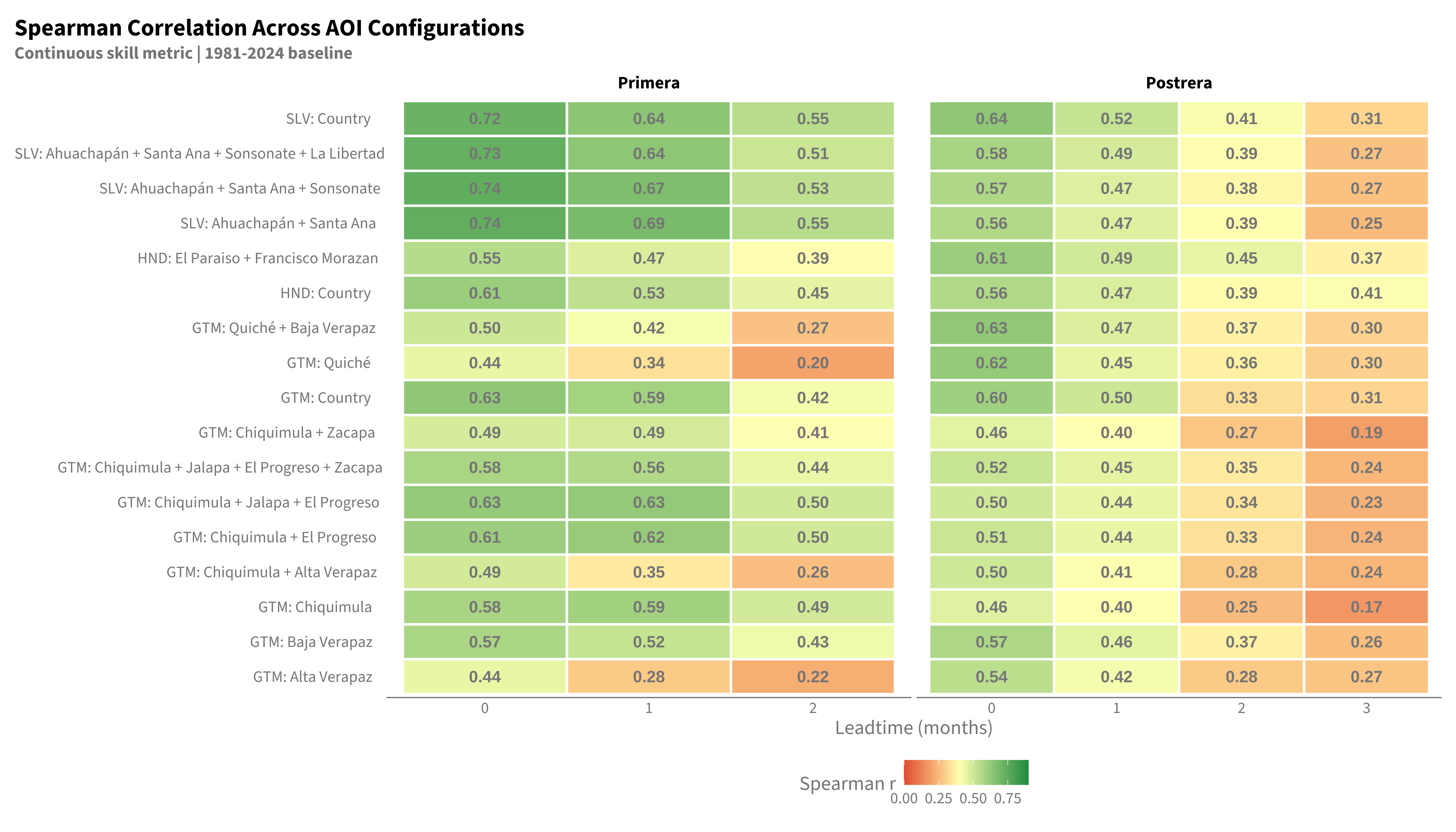
    title = "Spearman Correlation Across AOI Configurations",
    subtitle = "Continuous skill metric | 1981-2024 baseline",
    x = "Leadtime (months)", y = NULL
  ) +
  theme(panel.grid = element_blank())

8.4.4 Summary Table

8.4.5 Full Summary Table

8.5 RP3 vs RP4 Drought Definition

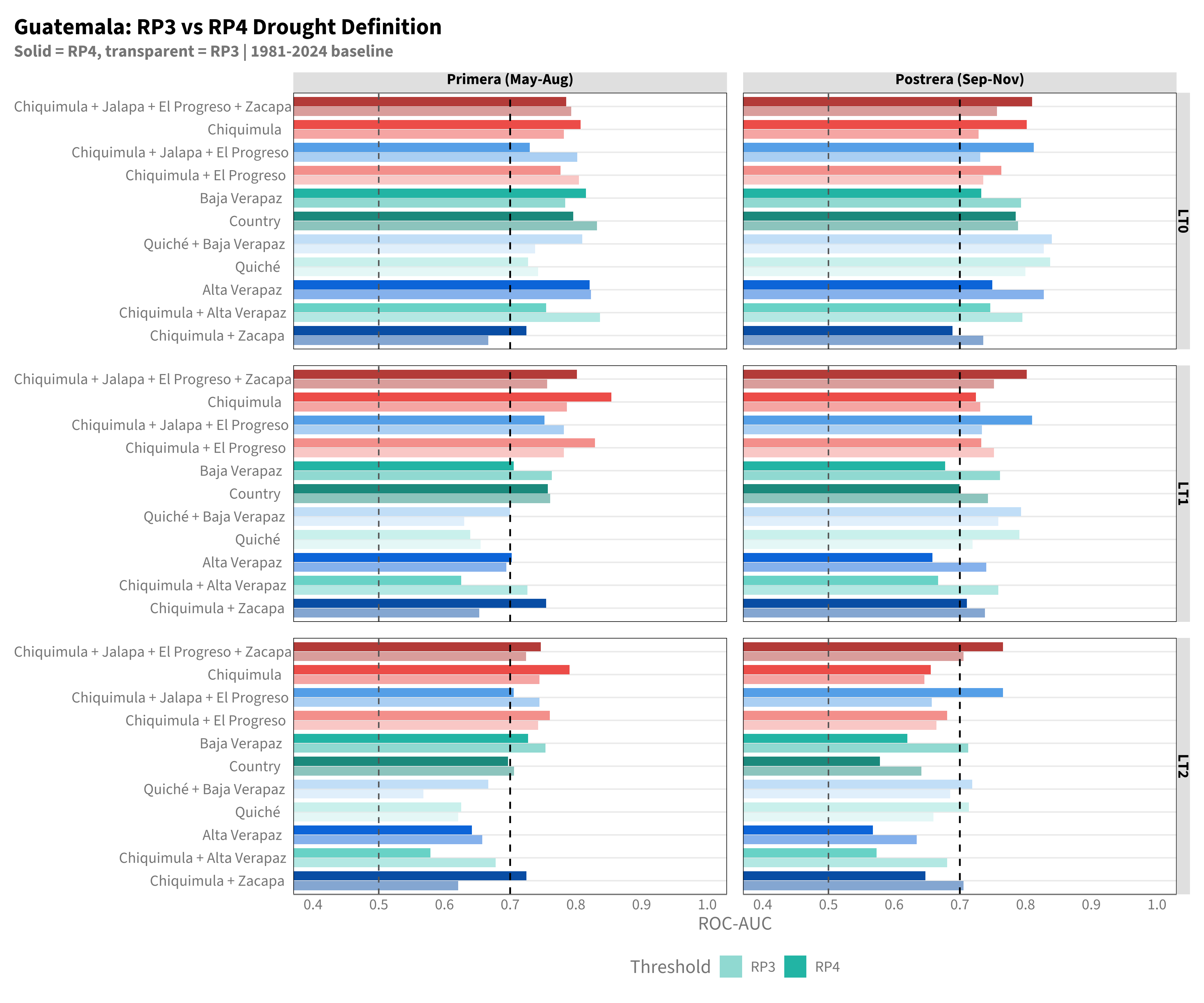
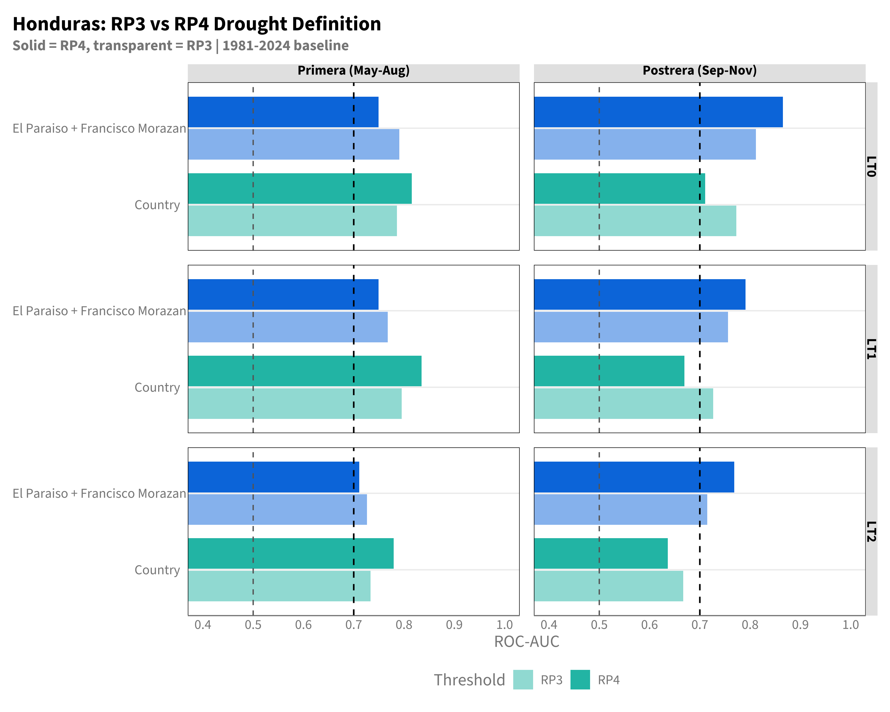
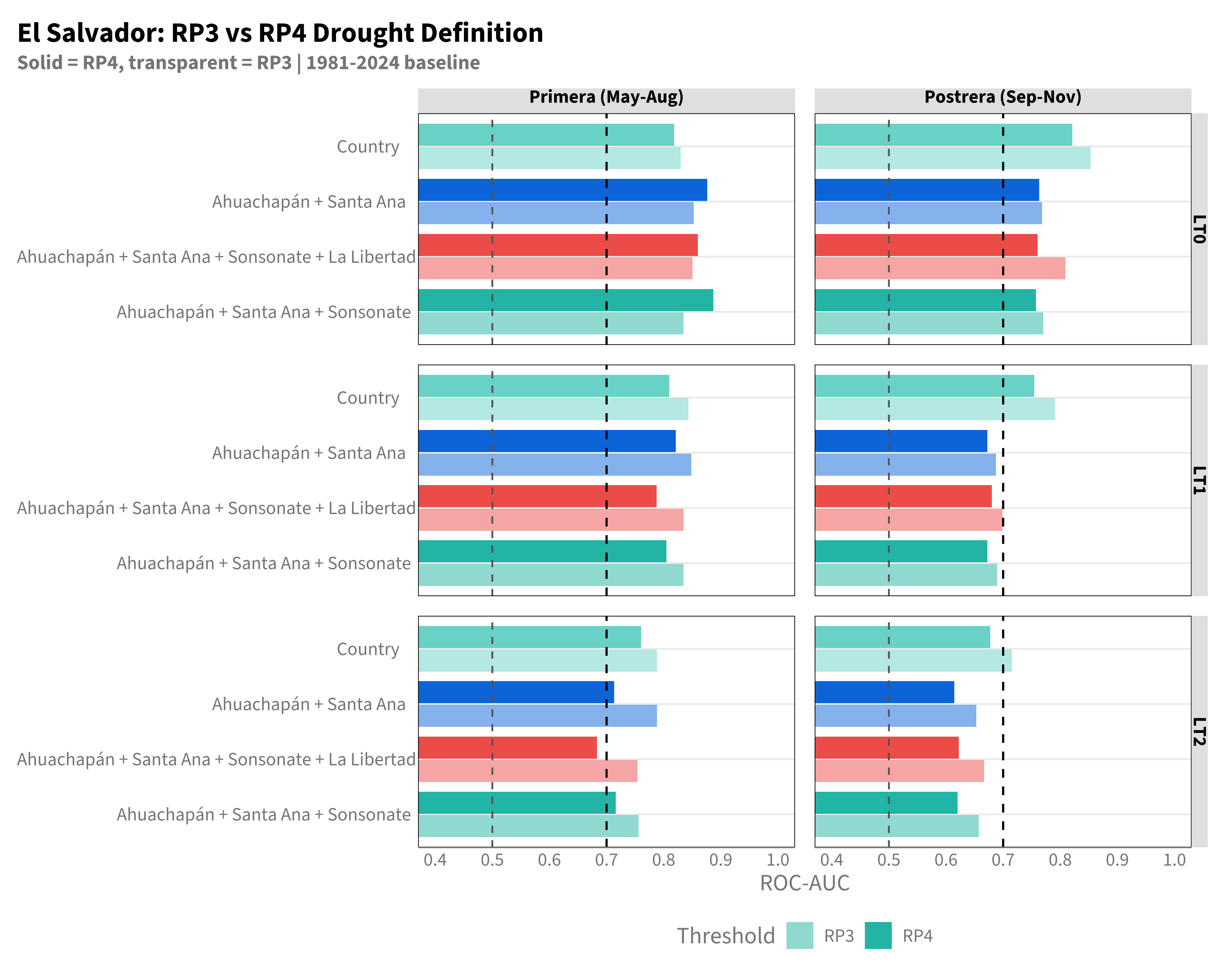
How sensitive are the results to the drought definition? Here we compare RP4 (1 in 4 year, ~25% of years) with RP3 (1 in 3 year, ~33% of years).

df_skill_rp3 <- calc_skill_metrics(df_all_configs, rp_target = 3) |> mutate(rp = "RP3")
df_skill_rp4 <- df_skill_admin |> mutate(rp = "RP4")
df_skill_rp_comparison <- bind_rows(df_skill_rp3, df_skill_rp4)

Guatemala

df_skill_rp_comparison |>
  filter(str_starts(aoi_config, "GTM"),
         (window == "primera" & leadtime %in% 0:2) |
         (window == "postrera" & leadtime %in% 0:2)) |>
  mutate(
    window_label = factor(window,
      levels = c("primera", "postrera"),
      labels = c("Primera (May-Aug)", "Postrera (Sep-Nov)")
    ),
    lt_label = paste0("LT", leadtime),
    aoi_label = str_remove(aoi_config, "^GTM: ")
  ) |>
  ggplot(aes(x = roc_auc, y = reorder(aoi_label, roc_auc), fill = aoi_label, alpha = rp)) +
  geom_col(position = position_dodge(width = 0.85), width = 0.8) +
  geom_vline(xintercept = 0.5, linetype = "dashed", color = "grey40") +
  geom_vline(xintercept = 0.7, linetype = "dashed", color = "black", linewidth = 0.6) +
  facet_grid(lt_label ~ window_label) +
  scale_alpha_manual(values = c("RP3" = 0.5, "RP4" = 1)) +
  scale_x_continuous(breaks = seq(0.4, 1, 0.1)) +
  coord_cartesian(xlim = c(0.4, 1)) +
  labs(
    title = "Guatemala: RP3 vs RP4 Drought Definition",
    subtitle = "Solid = RP4, transparent = RP3 | 1981-2024 baseline",
    x = "ROC-AUC", y = NULL, alpha = "Threshold"
  ) +
  theme_facet_bars +
  theme(legend.position = "bottom") +
  guides(fill = "none", alpha = guide_legend(nrow = 1))

Honduras

df_skill_rp_comparison |>
  filter(str_starts(aoi_config, "HND"),
         (window == "primera" & leadtime %in% 0:2) |
         (window == "postrera" & leadtime %in% 0:2)) |>
  mutate(
    window_label = factor(window,
      levels = c("primera", "postrera"),
      labels = c("Primera (May-Aug)", "Postrera (Sep-Nov)")
    ),
    lt_label = paste0("LT", leadtime),
    aoi_label = str_remove(aoi_config, "^HND: ")
  ) |>
  ggplot(aes(x = roc_auc, y = reorder(aoi_label, roc_auc), fill = aoi_label, alpha = rp)) +
  geom_col(position = position_dodge(width = 0.85), width = 0.8) +
  geom_vline(xintercept = 0.5, linetype = "dashed", color = "grey40") +
  geom_vline(xintercept = 0.7, linetype = "dashed", color = "black", linewidth = 0.6) +
  facet_grid(lt_label ~ window_label) +
  scale_alpha_manual(values = c("RP3" = 0.5, "RP4" = 1)) +
  scale_x_continuous(breaks = seq(0.4, 1, 0.1)) +
  coord_cartesian(xlim = c(0.4, 1)) +
  labs(
    title = "Honduras: RP3 vs RP4 Drought Definition",
    subtitle = "Solid = RP4, transparent = RP3 | 1981-2024 baseline",
    x = "ROC-AUC", y = NULL, alpha = "Threshold"
  ) +
  theme_facet_bars +
  theme(legend.position = "bottom") +
  guides(fill = "none", alpha = guide_legend(nrow = 1))

El Salvador

df_skill_rp_comparison |>
  filter(str_starts(aoi_config, "SLV"),
         (window == "primera" & leadtime %in% 0:2) |
         (window == "postrera" & leadtime %in% 0:2)) |>
  mutate(
    window_label = factor(window,
      levels = c("primera", "postrera"),
      labels = c("Primera (May-Aug)", "Postrera (Sep-Nov)")
    ),
    lt_label = paste0("LT", leadtime),
    aoi_label = str_remove(aoi_config, "^SLV: ")
  ) |>
  ggplot(aes(x = roc_auc, y = reorder(aoi_label, roc_auc), fill = aoi_label, alpha = rp)) +
  geom_col(position = position_dodge(width = 0.85), width = 0.8) +
  geom_vline(xintercept = 0.5, linetype = "dashed", color = "grey40") +
  geom_vline(xintercept = 0.7, linetype = "dashed", color = "black", linewidth = 0.6) +
  facet_grid(lt_label ~ window_label) +
  scale_alpha_manual(values = c("RP3" = 0.5, "RP4" = 1)) +
  scale_x_continuous(breaks = seq(0.4, 1, 0.1)) +
  coord_cartesian(xlim = c(0.4, 1)) +
  labs(
    title = "El Salvador: RP3 vs RP4 Drought Definition",
    subtitle = "Solid = RP4, transparent = RP3 | 1981-2024 baseline",
    x = "ROC-AUC", y = NULL, alpha = "Threshold"
  ) +
  theme_facet_bars +
  theme(legend.position = "bottom") +
  guides(fill = "none", alpha = guide_legend(nrow = 1))

8.6 OCHA AOI Skill Summary

Table 8.1 shows forecast skill for the selected OCHA AOIs used in the trigger optimization chapter.

# Map OCHA AOI configs to friendly country names
ocha_aoi_map <- c(
  "HND: HN07+HN08"          = "Honduras",
  "GTM: GT20+GT21+GT02+GT19" = "Guatemala",
  "SLV: Country"             = "El Salvador"
)

# Relabel the keys using the same relabel_config function
ocha_aoi_map_relabeled <- setNames(
  ocha_aoi_map,
  map_chr(names(ocha_aoi_map), \(x) {
    if (x == "SLV: Country") x else relabel_config(x)
  })
)

df_ocha_skill <- df_skill_admin |>
  filter(aoi_config %in% names(ocha_aoi_map_relabeled)) |>
  mutate(country = ocha_aoi_map_relabeled[aoi_config]) |>
  filter(
    (window == "primera" & leadtime %in% 0:2) |
    (window == "postrera" & leadtime %in% 0:3)
  ) |>
  mutate(
    score = sprintf("%.2f (%.2f)", roc_auc, f1),
    lt_label = paste0("LT", leadtime),
    window = factor(
      case_when(
        window == "primera" ~ "Primera (May\u2013Aug)",
        window == "postrera" ~ "Postrera (Sep\u2013Nov)"
      ),
      levels = c("Primera (May\u2013Aug)", "Postrera (Sep\u2013Nov)")
    )
  ) |>
  select(country, window, lt_label, score) |>
  pivot_wider(names_from = lt_label, values_from = score) |>
  arrange(window, country)

# Row indices (1-based within each group) for highlight targeting
primera_rows <- which(df_ocha_skill$window == "Primera (May\u2013Aug)")
postrera_rows <- which(df_ocha_skill$window == "Postrera (Sep\u2013Nov)")
postrera_gtm_hnd <- postrera_rows[df_ocha_skill$country[postrera_rows] %in% c("Guatemala", "Honduras")]
postrera_slv <- postrera_rows[df_ocha_skill$country[postrera_rows] == "El Salvador"]

df_ocha_skill |>
  gt(groupname_col = "window") |>
  tab_header(
    title = md("**SEAS5 Forecast Skill: ROC-AUC (F1)**"),
    subtitle = "RP4 drought threshold | 1981\u20132024 baseline | OCHA AOIs"
  ) |>
  cols_label(country = "Country") |>
  sub_missing(missing_text = "") |>
  # Highlight primera non-blank cells (LT0-LT2) green
  tab_style(
    style = cell_fill(color = "#d4edda"),
    locations = cells_body(columns = c(LT0, LT1, LT2), rows = primera_rows)
  ) |>
  # Highlight postrera LT0-2 for GTM & HND
  tab_style(
    style = cell_fill(color = "#d4edda"),
    locations = cells_body(columns = c(LT0, LT1, LT2), rows = postrera_gtm_hnd)
  ) |>
  # Highlight postrera LT0-1 for SLV
  tab_style(
    style = cell_fill(color = "#d4edda"),
    locations = cells_body(columns = c(LT0, LT1), rows = postrera_slv)
  ) |>
  tab_style(
    style = cell_text(weight = "bold", size = px(13)),
    locations = cells_row_groups()
  ) |>
  tab_style(
    style = cell_borders(sides = "bottom", color = "#dee2e6", weight = px(2)),
    locations = cells_column_labels()
  ) |>
  tab_footnote(
    footnote = "Format: ROC-AUC (F1). ROC-AUC > 0.7 = good; > 0.8 = excellent. Green = recommended leadtimes for trigger.",
    locations = cells_column_labels(columns = LT0)
  ) |>
  tab_options(
    table.font.size = px(14),
    heading.title.font.size = px(18),
    heading.subtitle.font.size = px(13),
    column_labels.font.weight = "bold",
    row_group.background.color = "#f8f9fa",
    table.border.top.style = "solid",
    table.border.top.width = px(2),
    table.border.top.color = "#1a9850"
  )

Table 8.1: SEAS5 Forecast Skill for OCHA AOIs

SEAS5 Forecast Skill: ROC-AUC (F1)
RP4 drought threshold | 1981–2024 baseline | OCHA AOIs
Country	LT01	LT1	LT2	LT3
Primera (May–Aug)
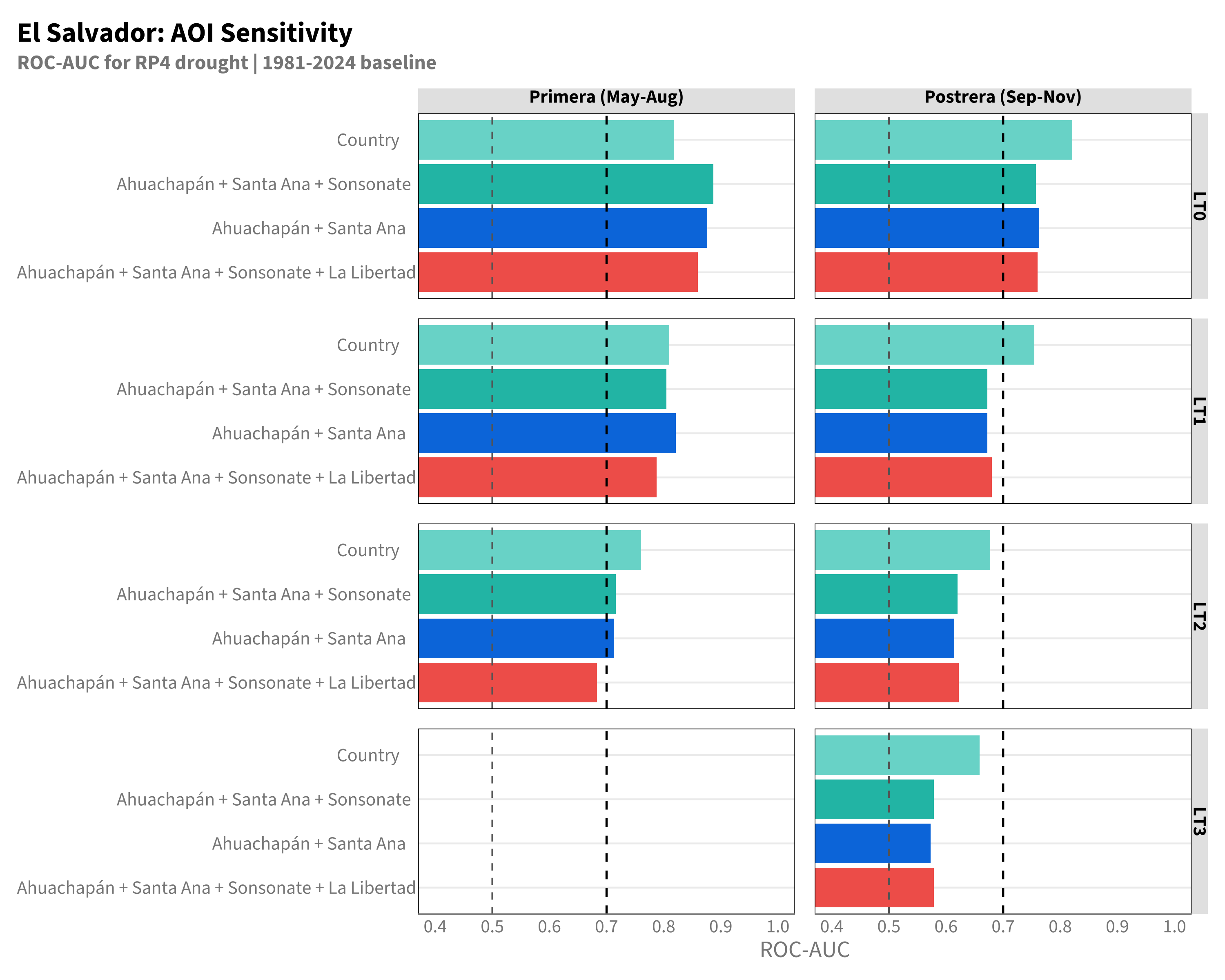
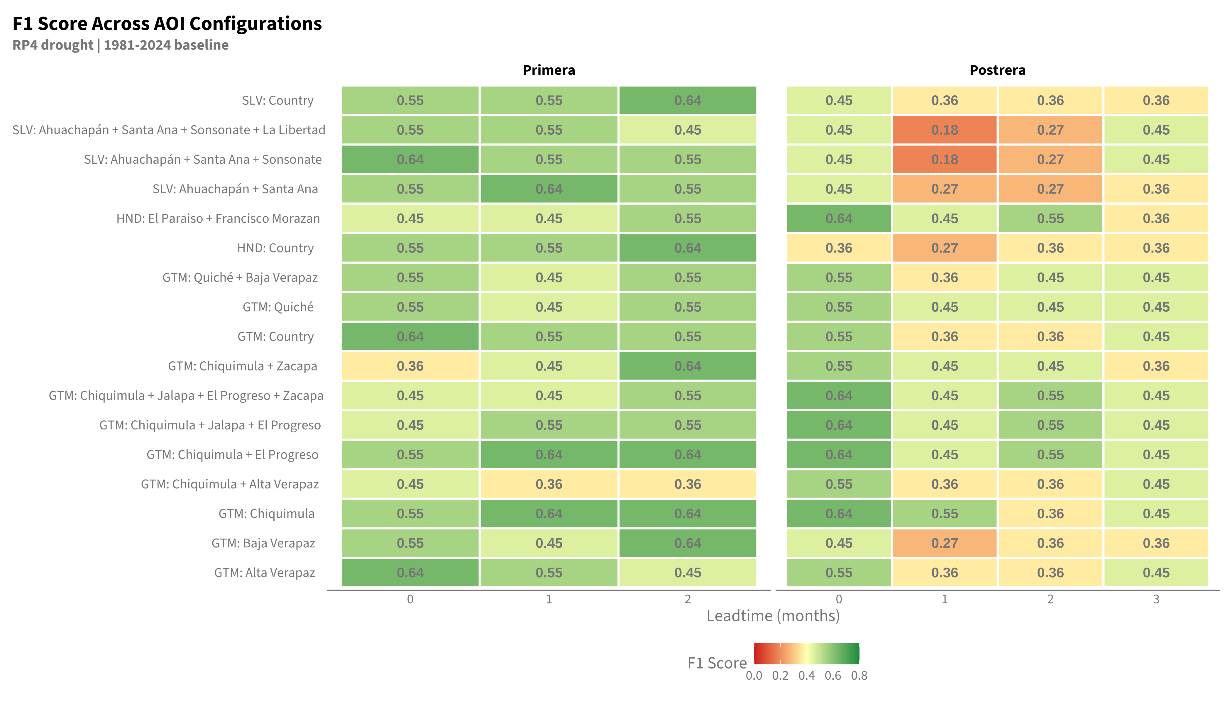
El Salvador	0.82 (0.55)	0.81 (0.55)	0.76 (0.64)
Guatemala	0.79 (0.45)	0.80 (0.45)	0.75 (0.55)
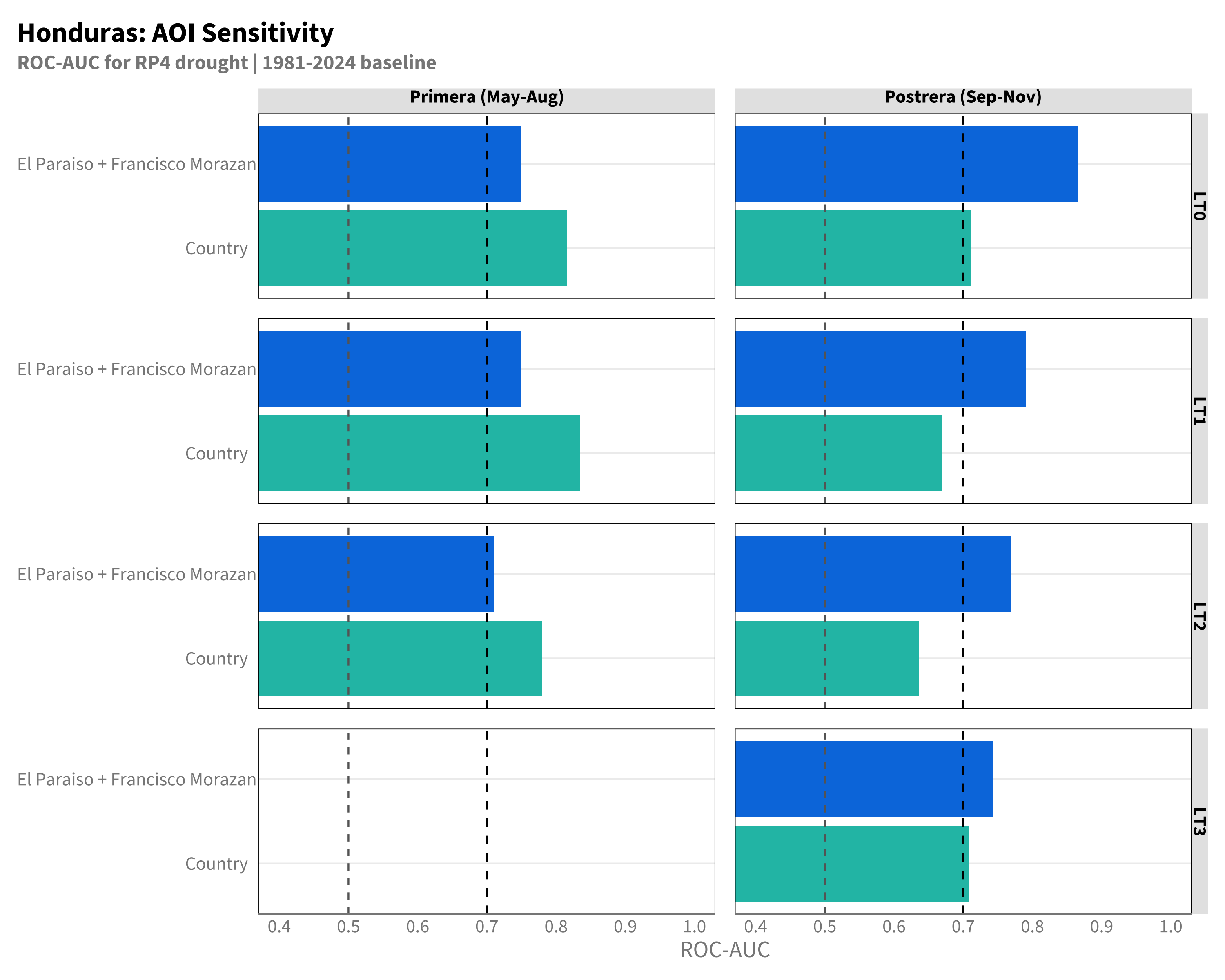
Honduras	0.75 (0.45)	0.75 (0.45)	0.71 (0.55)
Postrera (Sep–Nov)
El Salvador	0.82 (0.45)	0.75 (0.36)	0.68 (0.36)	0.66 (0.36)
Guatemala	0.81 (0.64)	0.80 (0.45)	0.77 (0.55)	0.75 (0.45)
Honduras	0.87 (0.64)	0.79 (0.45)	0.77 (0.55)	0.74 (0.36)
1 Format: ROC-AUC (F1). ROC-AUC > 0.7 = good; > 0.8 = excellent. Green = recommended leadtimes for trigger.

8.7 Start Network: Baja Verapaz & Quiché

NotePartner-specific analysis

The Start Network is exploring a separate trigger for Baja Verapaz (GT15) and Quiché (GT14). This section summarises the AOI skill assessment and recommended monitoring configuration. Detailed admin 2 decomposition is in Section 8.8.

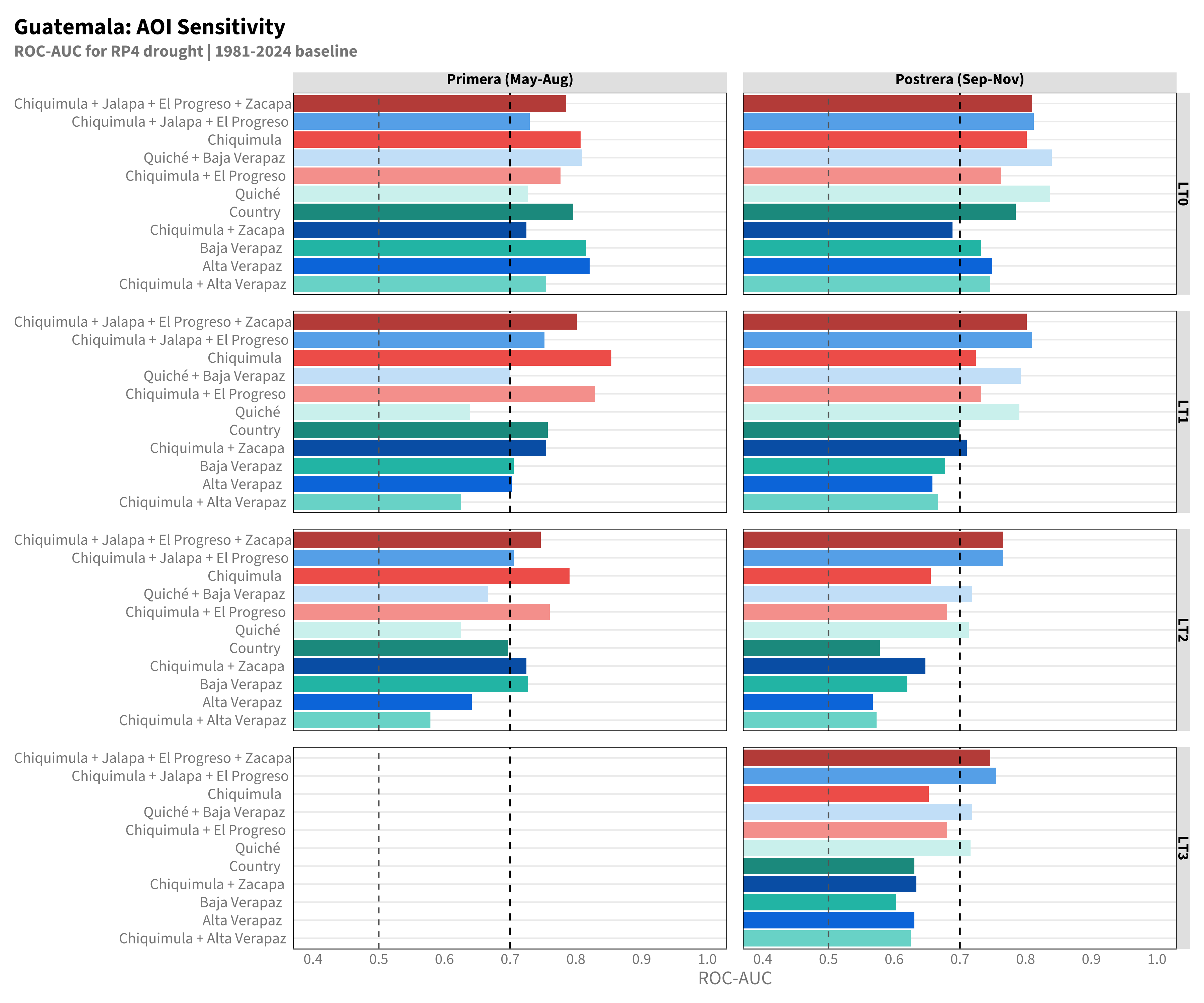
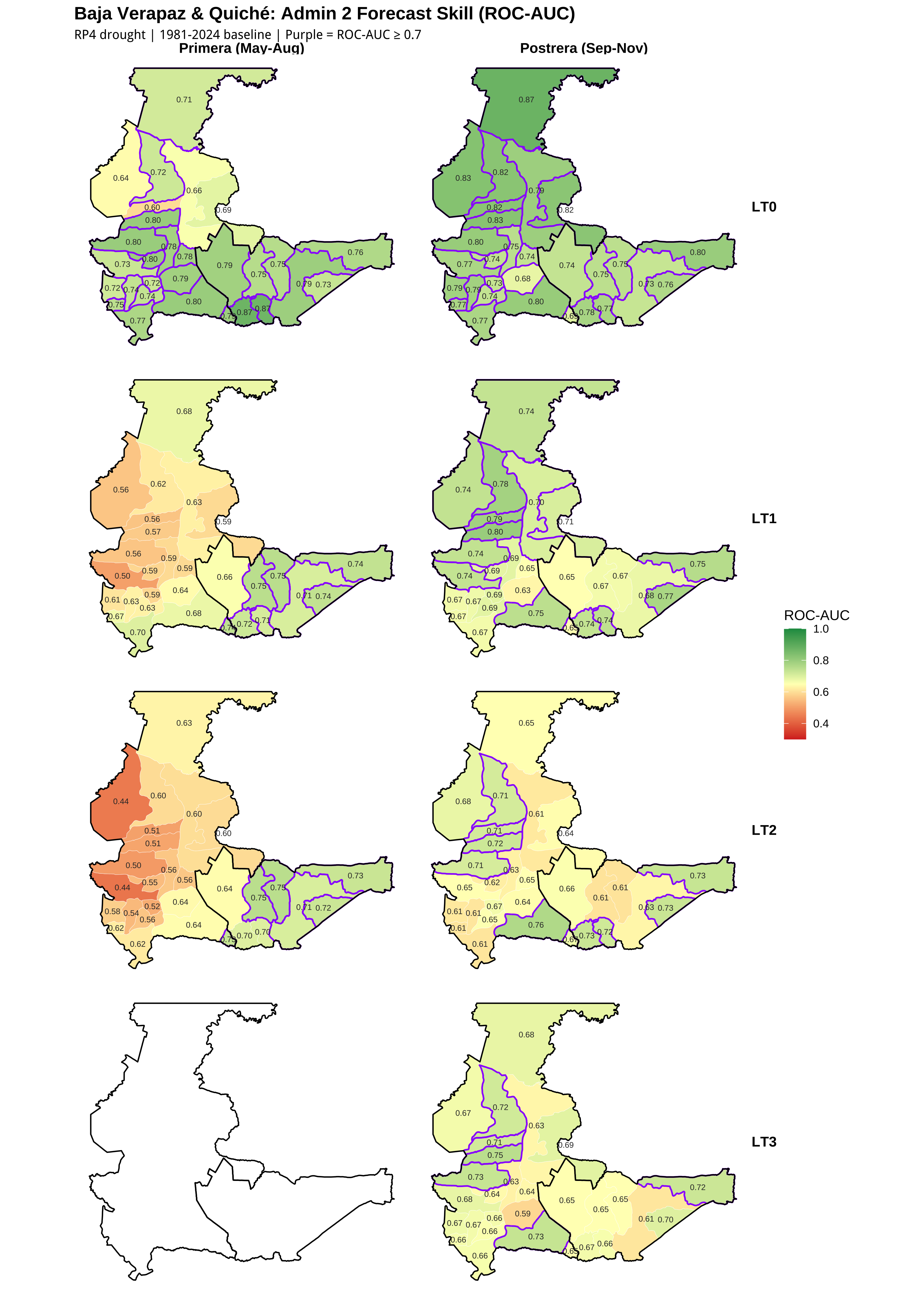
The Guatemala bar charts above already include Quiché, Baja Verapaz, and their combination (GT14+GT15). At the RP4 drought definition, the merged GT14+GT15 AOI exceeds ROC-AUC 0.7 at primera LT0 and LT1, and performs well for postrera. The main weak point is primera LT2, where the merged skill is dragged down by low-skill zones in northern Quiché. However, Baja Verapaz alone retains adequate skill at LT2.

ImportantRecommendation

For the Start Network trigger covering Baja Verapaz and Quiché:

• Primera LT0-LT1 and all postrera lead times: Use the merged GT14+GT15 AOI. The combined area has ROC-AUC above 0.7 at these lead times, and spatial averaging benefits skill.
• Primera LT2: Monitor Baja Verapaz (GT15) only. The merged AOI falls below acceptable skill at this lead time due to poorly-predicted zones in northern Quiché. If Baja Verapaz activates at primera LT2, the Start Network can still decide how best to prioritise resources between the two departments.

8.8 Appendix: Admin 2 Skill Decomposition for GT14+GT15

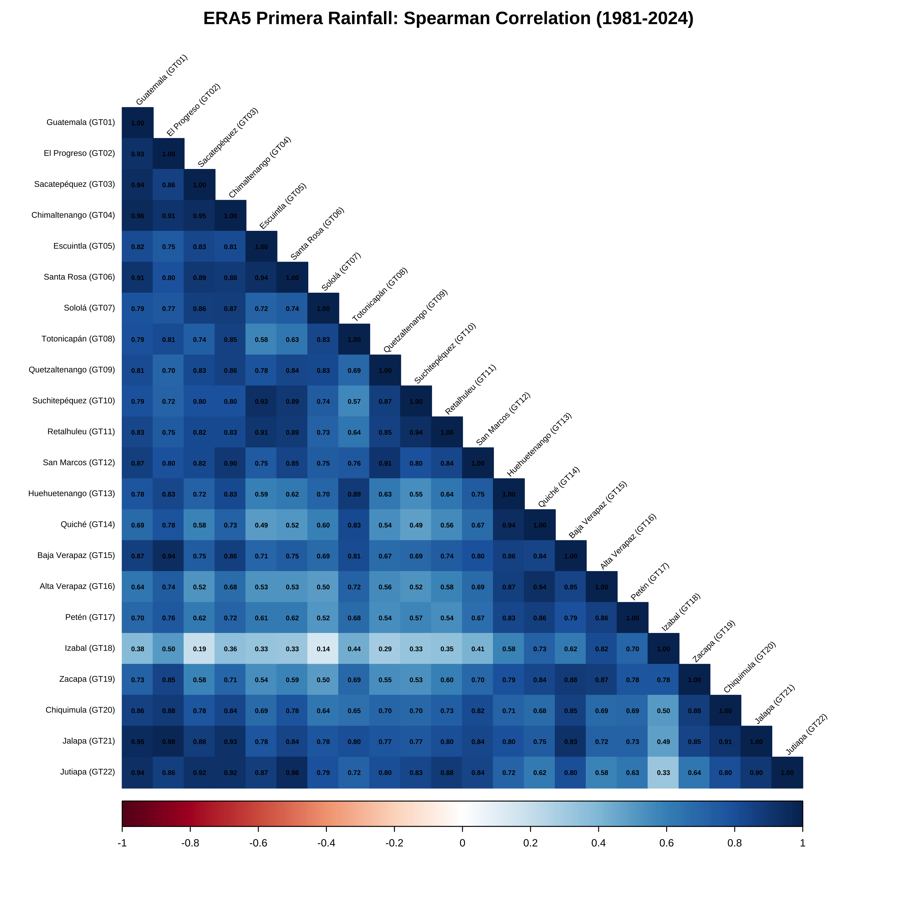
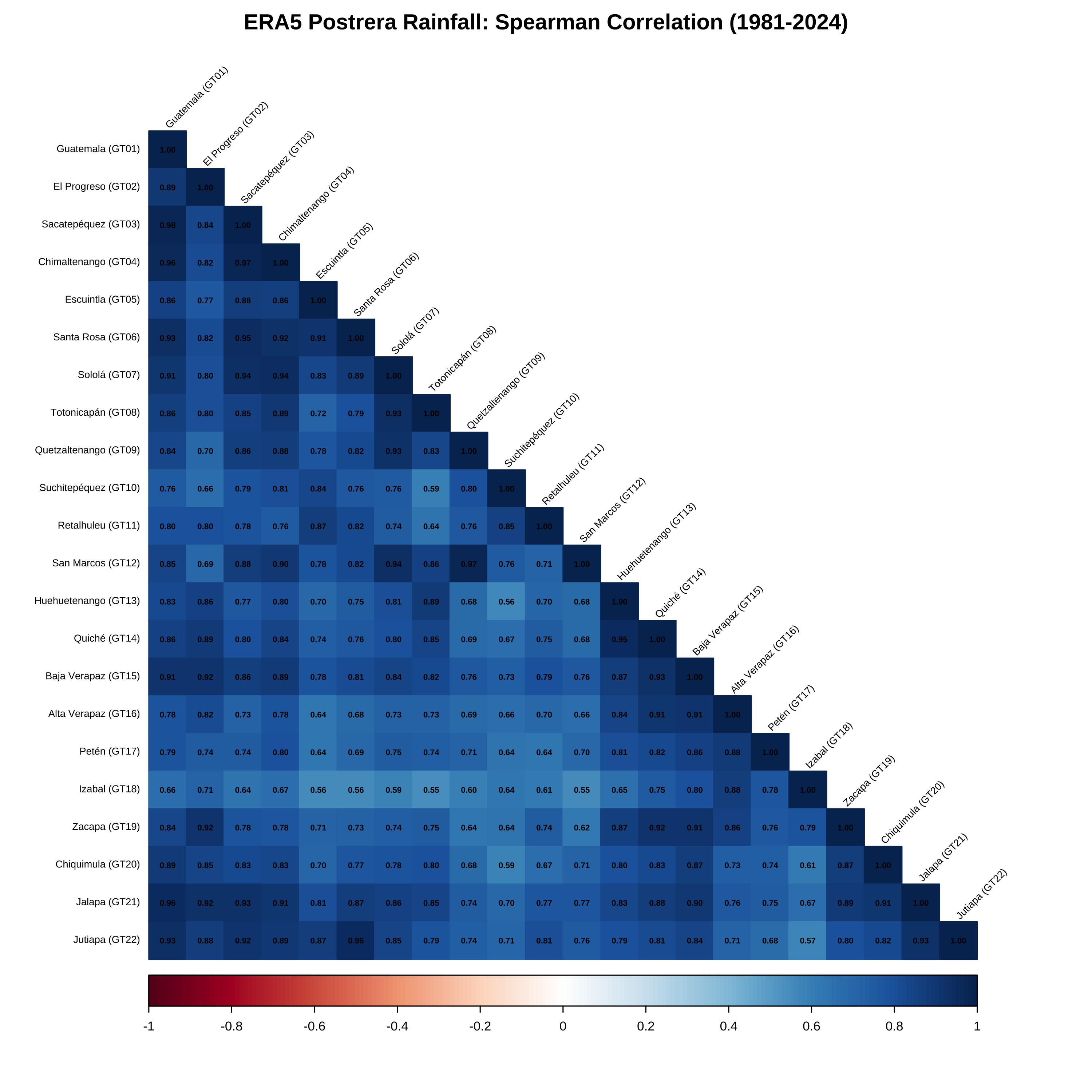
This appendix contains supplementary spatial analysis supporting the Start Network recommendation above, including inter-departmental rainfall correlation, admin 2-level forecast skill maps, leave-one-out decomposition, and forecast-similarity clustering.

8.8.1 Correlation Matrix

library(corrplot)

# Get department names from spatial data
name_col <- intersect(c("ADM1_ES", "adm1_es", "ADM1_EN", "adm1_en", "shapeName"), names(gdf_gtm))[1]
gtm_names <- gdf_gtm |>
  st_drop_geometry() |>
  rename(pcode = !!pcode_col, dept_name = !!name_col) |>
  select(pcode, dept_name) |>
  distinct()

for (szn in c("primera", "postrera")) {
  era5_wide <- df_gtm_seasonal |>
    filter(window == szn) |>
    left_join(gtm_names, by = "pcode") |>
    mutate(label = paste0(dept_name, " (", pcode, ")")) |>
    select(year, label, obs_mm) |>
    pivot_wider(names_from = label, values_from = obs_mm)

  cor_mat <- cor(era5_wide |> select(-year), method = "spearman", use = "complete.obs")

  corrplot(cor_mat, method = "color", type = "lower",
           tl.col = "black", tl.cex = 0.55, tl.srt = 45,
           addCoef.col = "black", number.cex = 0.45,
           cl.cex = 0.7, mar = c(0, 0, 2, 0),
           title = paste0("ERA5 ", tools::toTitleCase(szn),
                          " Rainfall: Spearman Correlation (1981-2024)"))
}

Figure 8.1: Spearman rank correlation of ERA5 seasonal rainfall across all Guatemala admin 1 departments (1981-2024).

Figure 8.2: Spearman rank correlation of ERA5 seasonal rainfall across all Guatemala admin 1 departments (1981-2024).

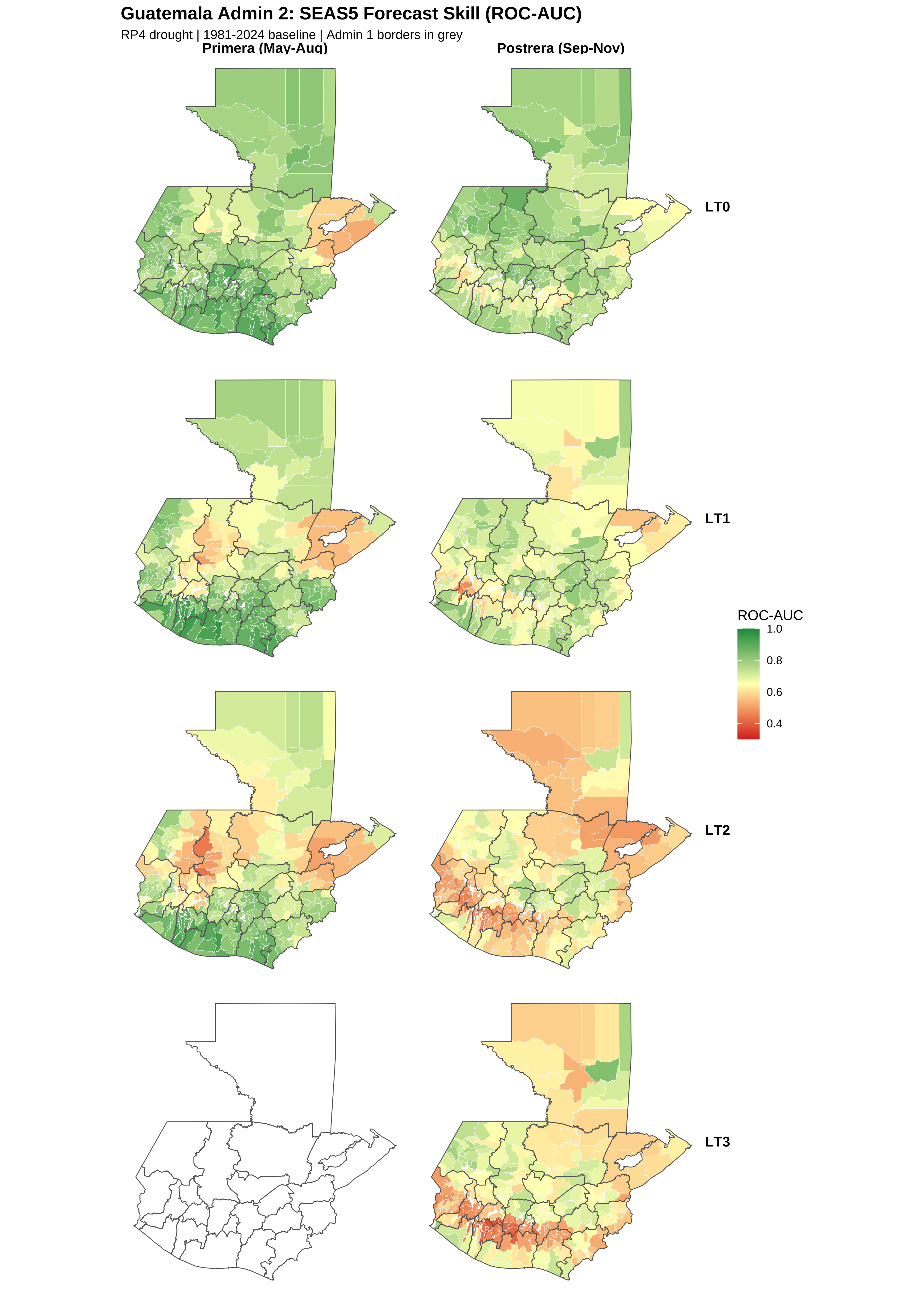
8.8.2 Admin 2 Forecast Skill Map

con <- pg_con()

df_seas5_gtm_adm2 <- tbl(con, "seas5") |>
  mutate(across(pcode, as.character)) |>
  filter(iso3 == "GTM", adm_level == 2) |>
  collect()

df_era5_gtm_adm2 <- tbl(con, "era5") |>
  mutate(across(pcode, as.character)) |>
  filter(iso3 == "GTM", adm_level == 2) |>
  collect()

DBI::dbDisconnect(con)

gdf_gtm_adm2 <- cumulus::download_fieldmaps_sf(iso3 = "gtm", layer = "gtm_adm2")$gtm_adm2

# Process to seasonal totals
df_seas5_adm2_mm <- df_seas5_gtm_adm2 |>
  mutate(value_mm = days_in_month(valid_date) * mean)

df_seas5_adm2_seasonal <- bind_rows(
  seas5_aggregate_forecast(df_seas5_adm2_mm, value = "value_mm",
    valid_months = PRIMERA_MONTHS,
    by = c("iso3", "pcode", "issued_date")) |> mutate(window = "primera"),
  seas5_aggregate_forecast(df_seas5_adm2_mm, value = "value_mm",
    valid_months = POSTRERA_MONTHS,
    by = c("iso3", "pcode", "issued_date")) |> mutate(window = "postrera")
) |>
  rename(fcst_mm = value_mm) |>
  mutate(year = year(issued_date), issued_month = month(issued_date)) |>
  filter(
    (window == "primera" & issued_month %in% PRIMERA_ISSUED_MONTHS) |
    (window == "postrera" & issued_month %in% POSTRERA_ISSUED_MONTHS)
  )

df_era5_adm2_monthly <- df_era5_gtm_adm2 |>
  mutate(year = year(valid_date), month = month(valid_date),
         value_mm = mean * days_in_month(valid_date))

df_era5_adm2_seasonal <- bind_rows(
  df_era5_adm2_monthly |>
    filter(month %in% PRIMERA_MONTHS) |>
    group_by(pcode, iso3, year) |>
    summarise(obs_mm = sum(value_mm), .groups = "drop") |>
    mutate(window = "primera"),
  df_era5_adm2_monthly |>
    filter(month %in% POSTRERA_MONTHS) |>
    group_by(pcode, iso3, year) |>
    summarise(obs_mm = sum(value_mm), .groups = "drop") |>
    mutate(window = "postrera")
)

df_adm2_joined <- df_seas5_adm2_seasonal |>
  left_join(df_era5_adm2_seasonal |> select(pcode, year, window, obs_mm),
            by = c("pcode", "year", "window")) |>
  filter(!is.na(obs_mm))

# Compute ROC-AUC per pcode/window/leadtime
drought_levels <- c("drought", "no_drought")
baseline_start <- 1981
baseline_end <- 2024
rp_target <- 4

df_adm2_baseline <- df_adm2_joined |>
  filter(year >= baseline_start, year <= baseline_end)

obs_thresh_adm2 <- df_adm2_baseline |>
  group_by(pcode, window) |>
  summarise(obs_thresh = calc_rp_threshold(obs_mm, rp_target, -1), .groups = "drop")

fcst_thresh_adm2 <- df_adm2_baseline |>
  group_by(pcode, window, leadtime) |>
  summarise(fcst_thresh = calc_rp_threshold(fcst_mm, rp_target, -1), .groups = "drop")

df_adm2_skill <- df_adm2_baseline |>
  left_join(obs_thresh_adm2, by = c("pcode", "window")) |>
  left_join(fcst_thresh_adm2, by = c("pcode", "window", "leadtime")) |>
  mutate(
    truth = fct(if_else(obs_mm <= obs_thresh, "drought", "no_drought"),
                levels = drought_levels),
    estimate = fct(if_else(fcst_mm <= fcst_thresh, "drought", "no_drought"),
                   levels = drought_levels)
  ) |>
  filter(!is.na(truth), !is.na(estimate)) |>
  group_by(pcode, window, leadtime) |>
  summarise(
    roc_auc = tryCatch(roc_auc_vec(truth, -fcst_mm, event_level = "first"),
                       error = function(e) NA_real_),
    .groups = "drop"
  )

# Normalise leadtime per window
df_adm2_skill <- df_adm2_skill |>
  group_by(window) |>
  mutate(leadtime = leadtime - min(leadtime)) |>
  ungroup()

pcode_col_adm2 <- intersect(c("ADM2_PCODE", "adm2_pcode", "pcode"), names(gdf_gtm_adm2))[1]

gdf_adm2_skill <- gdf_gtm_adm2 |>
  rename(pcode = !!pcode_col_adm2) |>
  left_join(df_adm2_skill, by = "pcode") |>
  filter(!is.na(window)) |>
  mutate(
    window_label = factor(window,
      levels = c("primera", "postrera"),
      labels = c("Primera (May-Aug)", "Postrera (Sep-Nov)")
    ),
    lt_label = paste0("LT", leadtime)
  )

# Admin 1 borders for reference
gdf_adm1_border <- gdf_gtm |>
  rename(pcode = !!pcode_col) |>
  st_union() |>
  st_cast("MULTILINESTRING")

ggplot(gdf_adm2_skill) +
  geom_sf(aes(fill = roc_auc), color = "white", linewidth = 0.1) +
  geom_sf(data = gdf_gtm |> rename(pcode = !!pcode_col),
          fill = NA, color = "grey40", linewidth = 0.3) +
  facet_grid(lt_label ~ window_label) +
  scale_fill_gradient2(
    low = "#D73027", mid = "#FFFFBF", high = "#1A9850",
    midpoint = 0.65, limits = c(0.3, 1), name = "ROC-AUC",
    oob = scales::squish, na.value = "grey90"
  ) +
  labs(
    title = "Guatemala Admin 2: SEAS5 Forecast Skill (ROC-AUC)",
    subtitle = "RP4 drought | 1981-2024 baseline | Admin 1 borders in grey"
  ) +
  theme_void() +
  theme(
    strip.text = element_text(size = 11, face = "bold"),
    legend.position = "right",
    plot.title = element_text(size = 14, face = "bold"),
    plot.subtitle = element_text(size = 10)
  )

Figure 8.3: ROC-AUC for predicting 1-in-4 year drought at admin 2 level across Guatemala (1981-2024).

# Filter to admin 2s within Baja Verapaz (GT15) and Quiché (GT14)
zoom_adm1 <- c("GT14", "GT15")
gdf_zoom <- gdf_adm2_skill |>
  filter(substr(pcode, 1, 4) %in% zoom_adm1)

# Subset with high skill for purple highlight
gdf_high_skill <- gdf_zoom |> filter(roc_auc >= 0.7)

# Admin 1 borders within zoom area
gdf_adm1_zoom <- gdf_gtm |>
  rename(pcode = !!pcode_col) |>
  filter(pcode %in% zoom_adm1)

# Centroid labels with ROC-AUC score
gdf_zoom_centroids <- st_centroid(gdf_zoom) |>
  mutate(roc_label = sprintf("%.2f", roc_auc))

ggplot(gdf_zoom) +
  geom_sf(aes(fill = roc_auc), color = "white", linewidth = 0.1) +
  geom_sf(data = gdf_high_skill, fill = NA, color = "#9B30FF", linewidth = 0.6) +
  geom_sf(data = gdf_adm1_zoom, fill = NA, color = "black", linewidth = 0.5, alpha = 0.4) +
  geom_sf_text(data = gdf_zoom_centroids, aes(label = roc_label),
               size = 2.2, color = "grey20") +
  facet_grid(lt_label ~ window_label) +
  scale_fill_gradient2(
    low = "#D73027", mid = "#FFFFBF", high = "#1A9850",
    midpoint = 0.65, limits = c(0.3, 1), name = "ROC-AUC",
    oob = scales::squish, na.value = "grey90"
  ) +
  labs(
    title = "Baja Verapaz & Quiché: Admin 2 Forecast Skill (ROC-AUC)",
    subtitle = "RP4 drought | 1981-2024 baseline | Purple = ROC-AUC \u2265 0.7"
  ) +
  theme_void() +
  theme(
    strip.text = element_text(size = 11, face = "bold"),
    legend.position = "right",
    plot.title = element_text(size = 14, face = "bold"),
    plot.subtitle = element_text(size = 10)
  )

Figure 8.4: ROC-AUC zoomed to Baja Verapaz & Quiché. Purple borders highlight admin 2 zones with ROC-AUC >= 0.7.

# Admin 2 pixel weights for GT14+GT15
con <- pg_con()
df_weights_adm2 <- tbl(con, "polygon") |>
  mutate(across(pcode, as.character)) |>
  filter(adm_level == 2, iso3 == "GTM") |>
  select(pcode, seas5_n_upsampled_pixels) |>
  collect() |>
  filter(substr(pcode, 1, 4) %in% c("GT14", "GT15"))
DBI::dbDisconnect(con)

sn_adm1 <- c("GT14", "GT15")

# Filter admin 2 joined data to GT14+GT15 (already loaded from earlier chunks)
df_sn_joined <- df_adm2_joined |>
  filter(substr(pcode, 1, 4) %in% sn_adm1) |>
  filter(year >= 1981, year <= 2024) |>
  group_by(window) |>
  mutate(leadtime = leadtime - min(leadtime)) |>
  ungroup()

sn_all_pcodes <- unique(df_sn_joined$pcode)
cat(sprintf("Admin 2 zones in GT14+GT15: %d\n", length(sn_all_pcodes)))

Admin 2 zones in GT14+GT15: 29

8.8.3 Per-LT Leave-One-Out: Primera Offenders

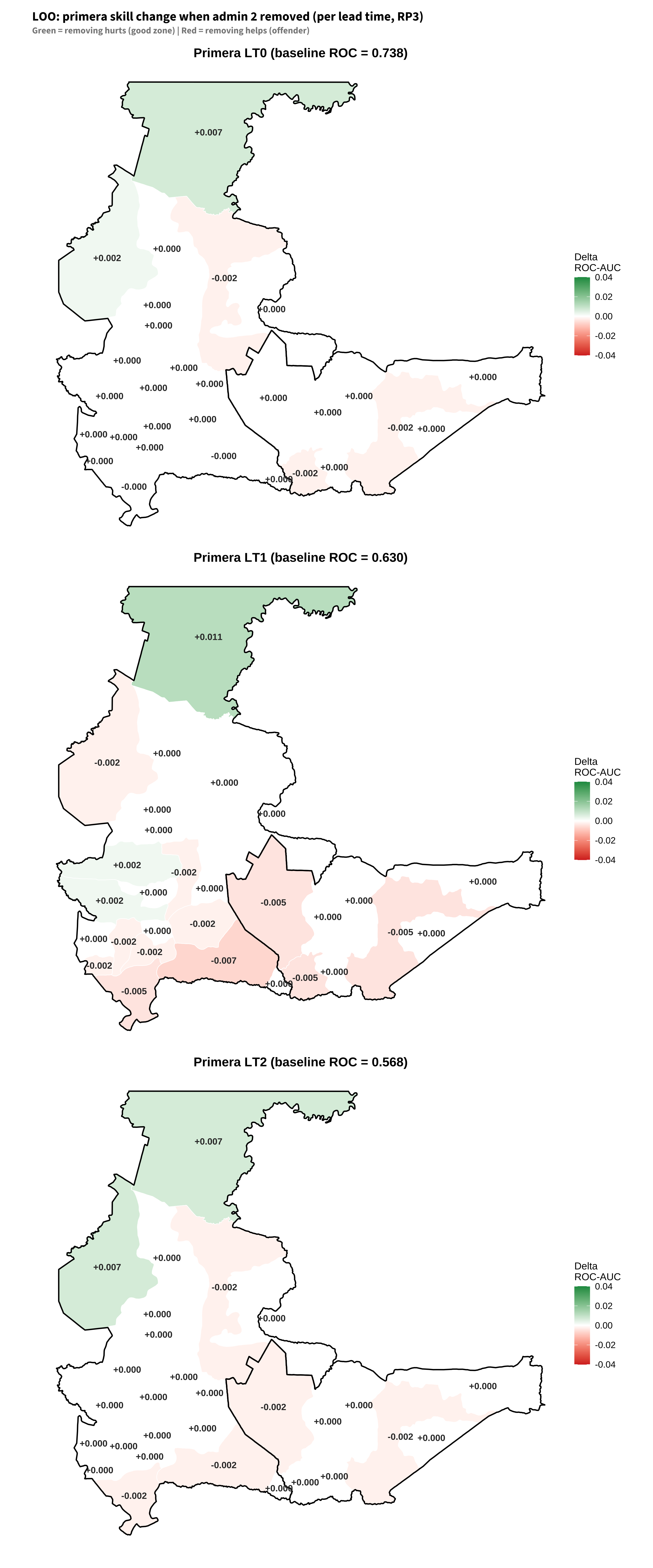
For each primera lead time, we compute the change in merged ROC-AUC when each admin 2 zone is removed. Green zones are contributors (removing them hurts); red zones are offenders (removing them helps). Individual LOO deltas are small because the offending zones are spatially clustered and share correlated forecast errors — removing one barely helps when its neighbours remain.

# Helper: merged ROC for single window-LT
sn_merged_roc <- function(pcodes, df_joined, df_weights,
                           rp_target = 3, target_window, target_lt) {
  df_m <- df_joined |>
    filter(pcode %in% pcodes, window == target_window, leadtime == target_lt) |>
    left_join(df_weights |> filter(pcode %in% pcodes), by = "pcode") |>
    group_by(year) |>
    summarise(
      fcst_mm = weighted.mean(fcst_mm, w = seas5_n_upsampled_pixels),
      obs_mm  = weighted.mean(obs_mm,  w = seas5_n_upsampled_pixels),
      .groups = "drop"
    )
  obs_thresh <- calc_rp_threshold(df_m$obs_mm, rp_target, -1)
  df_m <- df_m |>
    mutate(truth = fct(if_else(obs_mm <= obs_thresh, "drought", "no_drought"),
                       levels = c("drought", "no_drought")))
  tryCatch(roc_auc_vec(df_m$truth, -df_m$fcst_mm, event_level = "first"),
           error = function(e) NA_real_)
}

primera_lts <- df_sn_joined |>
  filter(window == "primera") |> distinct(leadtime) |>
  arrange(leadtime) |> pull(leadtime)

# Baseline per LT
baseline_lt <- tibble(
  leadtime = primera_lts,
  baseline_roc = map_dbl(primera_lts, ~sn_merged_roc(
    sn_all_pcodes, df_sn_joined, df_weights_adm2, 3, "primera", .x))
)

# LOO per admin 2 per LT
loo_lt <- list()
for (pc in sn_all_pcodes) {
  remaining <- setdiff(sn_all_pcodes, pc)
  for (lt in primera_lts) {
    roc_without <- sn_merged_roc(remaining, df_sn_joined, df_weights_adm2, 3, "primera", lt)
    bl <- baseline_lt$baseline_roc[baseline_lt$leadtime == lt]
    loo_lt[[length(loo_lt) + 1]] <- tibble(
      pcode = pc, leadtime = lt, roc_without = roc_without,
      baseline_roc = bl, delta = roc_without - bl
    )
  }
}

df_sn_loo <- bind_rows(loo_lt) |>
  mutate(lt_label = paste0("LT", leadtime))

# Spatial data already loaded
pcode_col_adm2 <- intersect(c("ADM2_PCODE", "adm2_pcode", "pcode"), names(gdf_gtm_adm2))[1]
gdf_sn <- gdf_gtm_adm2 |>
  rename(pcode = !!pcode_col_adm2) |>
  filter(substr(pcode, 1, 4) %in% sn_adm1)

gdf_sn_adm1 <- gdf_gtm |>
  rename(pcode = !!pcode_col) |>
  filter(pcode %in% sn_adm1)

loo_maps <- list()
for (lt in primera_lts) {
  gdf_lt <- gdf_sn |>
    left_join(df_sn_loo |> filter(leadtime == lt) |> select(pcode, delta),
              by = "pcode")
  gdf_lt_c <- st_centroid(gdf_lt) |>
    mutate(delta_label = sprintf("%+.3f", delta))

  bl_roc <- baseline_lt$baseline_roc[baseline_lt$leadtime == lt]

  loo_maps[[paste0("LT", lt)]] <- ggplot(gdf_lt) +
    geom_sf(aes(fill = delta), color = "white", linewidth = 0.3) +
    geom_sf(data = gdf_sn_adm1, fill = NA, color = "black",
            linewidth = 0.7, alpha = 0.5) +
    geom_sf_text(data = gdf_lt_c, aes(label = delta_label),
                 size = 3.5, color = "grey20", fontface = "bold") +
    scale_fill_gradient2(
      low = "#D73027", mid = "white", high = "#1A9850",
      midpoint = 0, name = "Delta\nROC-AUC",
      limits = c(-0.04, 0.04), oob = scales::squish
    ) +
    labs(title = sprintf("Primera LT%d (baseline ROC = %.3f)", lt, bl_roc)) +
    theme_void() +
    theme(
      plot.title = element_text(size = 14, face = "bold", hjust = 0.5),
      legend.position = "right",
      legend.text = element_text(size = 10),
      legend.title = element_text(size = 11)
    )
}

patchwork::wrap_plots(loo_maps, ncol = 1) +
  patchwork::plot_annotation(
    title = "LOO: primera skill change when admin 2 removed (per lead time, RP3)",
    subtitle = "Green = removing hurts (good zone) | Red = removing helps (offender)",
    theme = theme(
      plot.title = element_text(size = 14, face = "bold"),
      plot.subtitle = element_text(size = 10)
    )
  )

Figure 8.5: Leave-one-out primera skill impact per lead time (RP3 drought, 1981-2024). Green = removing zone hurts merged skill (good zone). Red = removing zone helps (offender).

8.8.4 Forecast Similarity Clustering

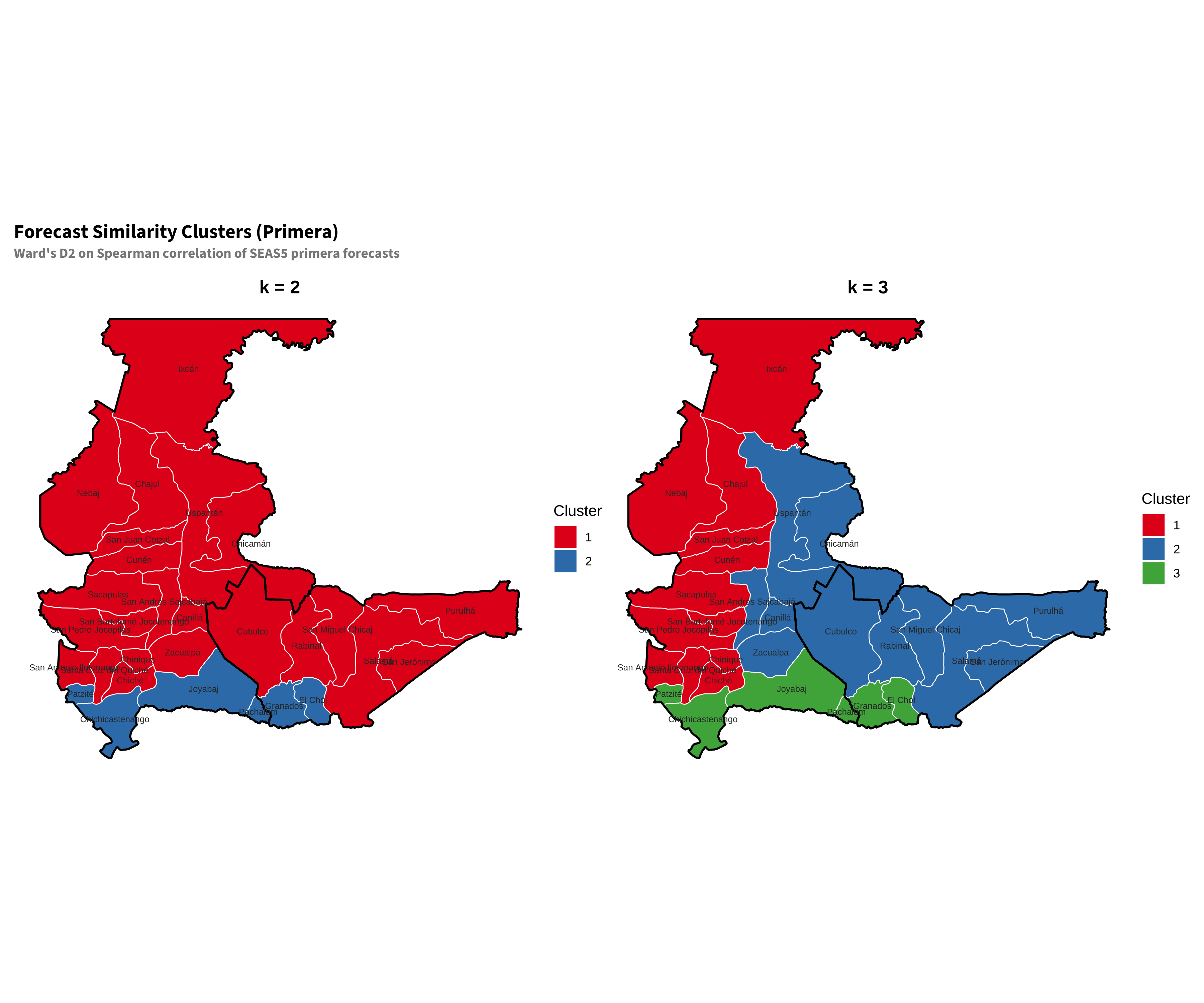
To address the limitation of single-zone LOO (offenders are spatially correlated, so individual deltas are tiny), we cluster admin 2 zones by forecast similarity and evaluate skill when entire clusters are removed.

We compute pairwise Spearman correlation of primera forecast time series across all admin 2 zones, then apply hierarchical clustering (Ward’s D2 on the distance matrix 1 - correlation). We evaluate cuts at k = 2 and k = 3 to find a partition that cleanly separates the low-skill block.

# Build primera forecast matrix: rows = years, cols = admin 2 zones
# Average across lead times for the clustering
df_primera_wide <- df_sn_joined |>
  filter(window == "primera") |>
  group_by(pcode, year) |>
  summarise(fcst_mm = mean(fcst_mm), .groups = "drop") |>
  pivot_wider(names_from = pcode, values_from = fcst_mm)

fcst_mat <- df_primera_wide |> select(-year) |> as.matrix()
rownames(fcst_mat) <- df_primera_wide$year

# Spearman correlation → distance → hierarchical clustering
cor_mat <- cor(fcst_mat, method = "spearman", use = "complete.obs")
dist_mat <- as.dist(1 - cor_mat)
hc <- hclust(dist_mat, method = "ward.D2")

# Get zone names column
sn_name_col <- intersect(
  c("ADM2_ES", "adm2_es", "ADM2_EN", "adm2_en", "shapeName"),
  names(gdf_sn)
)[1]

# Cut at k = 2 and k = 3
df_clusters_k2 <- tibble(pcode = names(cutree(hc, k = 2)),
                          cluster = cutree(hc, k = 2))
df_clusters_k3 <- tibble(pcode = names(cutree(hc, k = 3)),
                          cluster = cutree(hc, k = 3))

cluster_pal <- c(
  "1" = "#E41A1C", "2" = "#377EB8",
  "3" = "#4DAF4A", "4" = "#984EA3"
)

make_cluster_map <- function(df_cl, k_label) {
  gdf_cl <- gdf_sn |>
    left_join(df_cl, by = "pcode") |>
    mutate(cluster_label = factor(cluster))

  gdf_cl_c <- st_centroid(gdf_cl) |>
    rename(zone_name = !!sn_name_col)

  ggplot(gdf_cl) +
    geom_sf(aes(fill = cluster_label), color = "white", linewidth = 0.3) +
    geom_sf(data = gdf_sn_adm1, fill = NA, color = "black",
            linewidth = 0.7, alpha = 0.5) +
    geom_sf_text(data = gdf_cl_c, aes(label = zone_name),
                 size = 2.2, color = "grey20") +
    scale_fill_manual(values = cluster_pal, name = "Cluster", drop = FALSE) +
    labs(title = k_label) +
    theme_void() +
    theme(
      plot.title = element_text(size = 13, face = "bold", hjust = 0.5),
      legend.position = "right"
    )
}

p_k2 <- make_cluster_map(df_clusters_k2, "k = 2")
p_k3 <- make_cluster_map(df_clusters_k3, "k = 3")

patchwork::wrap_plots(p_k2, p_k3, ncol = 2) +
  patchwork::plot_annotation(
    title = "Forecast Similarity Clusters (Primera)",
    subtitle = "Ward's D2 on Spearman correlation of SEAS5 primera forecasts",
    theme = theme(
      plot.title = element_text(size = 14, face = "bold"),
      plot.subtitle = element_text(size = 10)
    )
  )

Figure 8.6: Admin 2 zones coloured by forecast similarity cluster at k=2 (left) and k=3 (right). Hierarchical clustering (Ward’s D2) on Spearman correlation of primera SEAS5 forecasts.

# For each k and each cluster, compute merged primera skill without it
build_cluster_configs <- function(df_cl, k_label) {
  configs <- list()

  # Individual cluster removal
  for (cl in sort(unique(df_cl$cluster))) {
    cl_zones <- df_cl |> filter(cluster == cl) |> pull(pcode)
    remaining <- setdiff(sn_all_pcodes, cl_zones)
    n_removed <- length(cl_zones)
    configs[[sprintf("%s: Drop CL%d (%d zones)", k_label, cl, n_removed)]] <- remaining
  }

  # Multi-cluster removal: all 2-cluster combos
  all_cls <- sort(unique(df_cl$cluster))
  if (length(all_cls) >= 2) {
    for (i in seq_along(all_cls)) {
      for (j in seq_along(all_cls)) {
        if (j <= i) next
        cl_i <- all_cls[i]; cl_j <- all_cls[j]
        cl_zones <- df_cl |> filter(cluster %in% c(cl_i, cl_j)) |> pull(pcode)
        remaining <- setdiff(sn_all_pcodes, cl_zones)
        if (length(remaining) < 4) next
        n_removed <- length(cl_zones)
        configs[[sprintf("%s: Drop CL%d+CL%d (%d zones)", k_label,
                         cl_i, cl_j, n_removed)]] <- remaining
      }
    }
  }

  configs
}

sn_cluster_configs <- c(
  list("All 29 zones (baseline)" = sn_all_pcodes),
  build_cluster_configs(df_clusters_k2, "k=2"),
  build_cluster_configs(df_clusters_k3, "k=3")
)

# Compute skill for each config
sn_cluster_skill <- list()
for (nm in names(sn_cluster_configs)) {
  pcs <- sn_cluster_configs[[nm]]
  for (lt in primera_lts) {
    roc_val <- sn_merged_roc(pcs, df_sn_joined, df_weights_adm2, 3, "primera", lt)
    sn_cluster_skill[[length(sn_cluster_skill) + 1]] <- tibble(
      config = nm, leadtime = lt, roc_auc = roc_val,
      n_zones = length(pcs)
    )
  }
}

df_cluster_skill <- bind_rows(sn_cluster_skill)

# Build cluster membership footnotes for both k values
make_cluster_footnote <- function(df_cl, k_label) {
  df_cl |>
    left_join(
      gdf_sn |> st_drop_geometry() |>
        select(pcode, any_of(sn_name_col)) |>
        rename(name = !!sn_name_col),
      by = "pcode"
    ) |>
    group_by(cluster) |>
    summarise(zones = paste(name, collapse = ", "), n = n(), .groups = "drop") |>
    mutate(label = sprintf("%s CL%d (%d): %s", k_label, cluster, n, zones)) |>
    pull(label) |>
    paste(collapse = ". ")
}

footnote_k2 <- make_cluster_footnote(df_clusters_k2, "k=2")
footnote_k3 <- make_cluster_footnote(df_clusters_k3, "k=3")

df_cluster_skill |>
  mutate(
    lt_label = paste0("LT", leadtime),
    roc_label = sprintf("%.3f", roc_auc)
  ) |>
  select(config, n_zones, lt_label, roc_label) |>
  pivot_wider(names_from = lt_label, values_from = roc_label) |>
  arrange(desc(n_zones)) |>
  gt() |>
  tab_header(
    title = md("**Leave-Cluster-Out: Primera Skill**"),
    subtitle = "ROC-AUC | RP3 drought | 1981-2024 baseline"
  ) |>
  cols_label(config = "Configuration", n_zones = "Zones") |>
  tab_footnote(footnote = footnote_k2) |>
  tab_footnote(footnote = footnote_k3)

Table 8.2: Leave-cluster-out analysis: primera ROC-AUC (RP3) when clusters are removed. Shown for k=2 and k=3 cuts of the dendrogram.

Leave-Cluster-Out: Primera Skill
ROC-AUC | RP3 drought | 1981-2024 baseline
Configuration	Zones	LT0	LT1	LT2
All 29 zones (baseline)	29	0.738	0.630	0.568
k=2: Drop CL2 (6 zones)	23	0.743	0.614	0.561
k=3: Drop CL3 (6 zones)	23	0.743	0.614	0.561
k=3: Drop CL2 (11 zones)	18	0.733	0.657	0.616
k=3: Drop CL1 (12 zones)	17	0.802	0.706	0.669
k=3: Drop CL2+CL3 (17 zones)	12	0.731	0.637	0.605
k=3: Drop CL1+CL3 (18 zones)	11	0.784	0.692	0.667
k=2: Drop CL1 (23 zones)	6	0.821	0.722	0.632
k=3: Drop CL1+CL2 (23 zones)	6	0.821	0.722	0.632
k=2 CL1 (23): Santa Cruz del Quiché, Chiché, Chinique, Zacualpa, Chajul, San Antonio Ilotenango, San Pedro Jocopilas, Cunén, San Juan Cotzal, Nebaj, San Andrés Sajcabajá, Uspantán, Sacapulas, San Bartolomé Jocotenango, Canillá, Chicamán, Ixcán, Salamá, San Miguel Chicaj, Rabinal, Cubulco, San Jerónimo, Purulhá. k=2 CL2 (6): Chichicastenango, Patzité, Joyabaj, Pachalum, Granados, El Chol
k=3 CL1 (12): Santa Cruz del Quiché, Chiché, Chinique, Chajul, San Antonio Ilotenango, San Pedro Jocopilas, Cunén, San Juan Cotzal, Nebaj, Sacapulas, San Bartolomé Jocotenango, Ixcán. k=3 CL2 (11): Zacualpa, San Andrés Sajcabajá, Uspantán, Canillá, Chicamán, Salamá, San Miguel Chicaj, Rabinal, Cubulco, San Jerónimo, Purulhá. k=3 CL3 (6): Chichicastenango, Patzité, Joyabaj, Pachalum, Granados, El Chol

The clustering confirms that the low-skill zones concentrate in a geographically coherent block in northern Quiché. However, no single cluster removal fully captures the set of offenders — the low-skill zones span multiple forecast-similarity clusters, and the spatial correlation of forecast errors makes automated selection difficult. This supports the simpler approach adopted in the main recommendation: use the merged AOI where skill is adequate (primera LT0-LT1, all postrera), and fall back to Baja Verapaz only for primera LT2.

8.8.5 Qualitative Admin 2 Removal

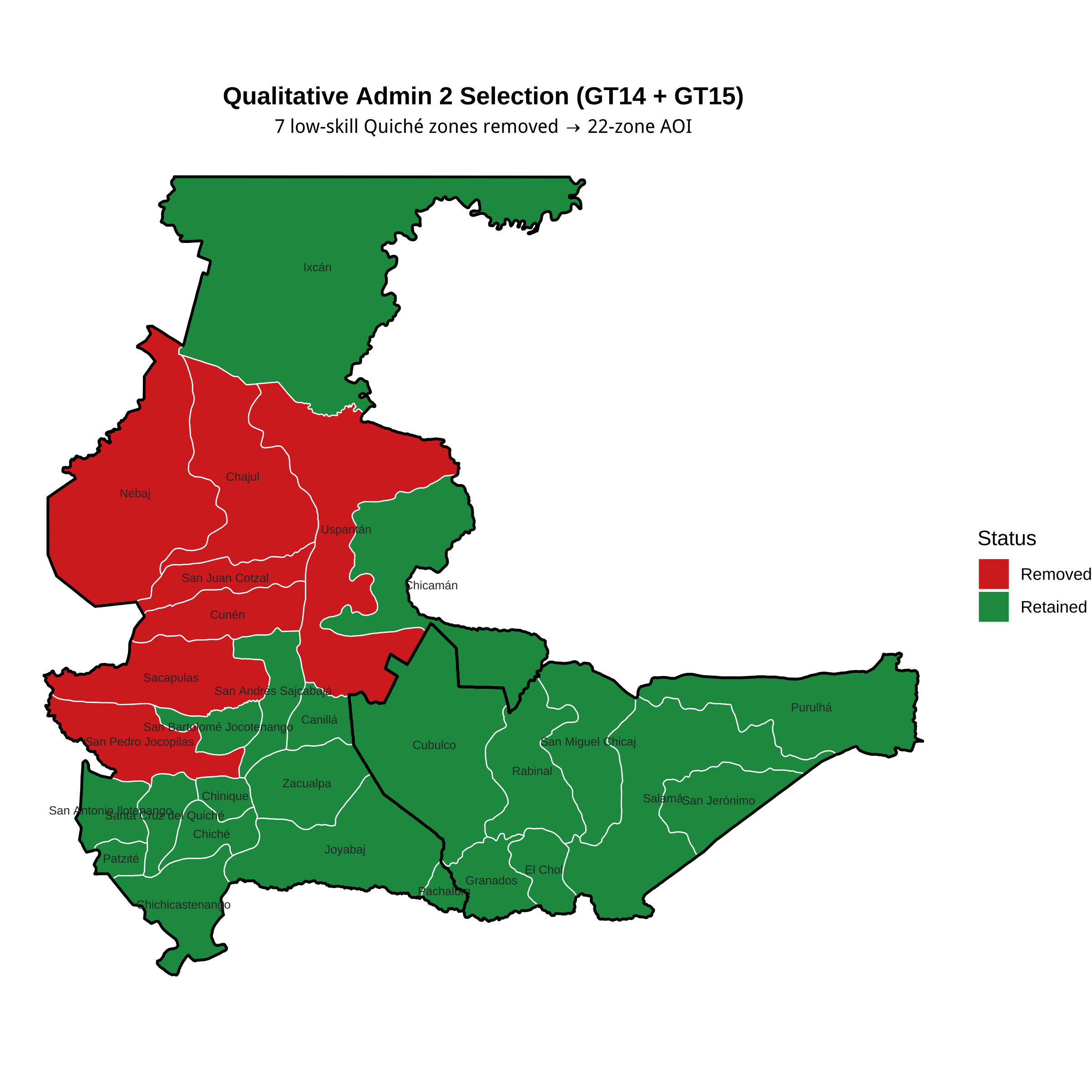
As an alternative to automated clustering, we manually identified 7 low-skill Quiché admin 2 zones informed by the LOO and greedy analyses above. Removing these zones yields a 22-zone AOI. The table below compares ROC-AUC across all lead times and seasons for three configurations: the full 29-zone merge, the 22-zone qualitative selection, and Baja Verapaz (GT15) only.

qual_remove <- c("GT1413", "GT1411", "GT1410", "GT1416", "GT1409", "GT1415", "GT1405")
qual_remaining <- setdiff(sn_all_pcodes, qual_remove)
gt15_only <- sn_all_pcodes[startsWith(sn_all_pcodes, "GT15")]

postrera_lts <- df_sn_joined |>
  filter(window == "postrera") |> distinct(leadtime) |>
  arrange(leadtime) |> pull(leadtime)

aoi_configs <- list(
  "All 29 zones (GT14+GT15)" = sn_all_pcodes,
  "22 zones (7 Quiché removed)" = qual_remaining,
  "GT15 only (Baja Verapaz)" = gt15_only
)

qual_results <- list()
for (rp in c(3, 4)) {
  for (nm in names(aoi_configs)) {
    pcs <- aoi_configs[[nm]]
    for (lt in primera_lts) {
      roc_val <- sn_merged_roc(pcs, df_sn_joined, df_weights_adm2, rp, "primera", lt)
      qual_results[[length(qual_results) + 1]] <- tibble(
        config = nm, rp_def = rp, window = "primera", leadtime = lt,
        roc_auc = roc_val, n_zones = length(pcs)
      )
    }
    for (lt in postrera_lts) {
      roc_val <- sn_merged_roc(pcs, df_sn_joined, df_weights_adm2, rp, "postrera", lt)
      qual_results[[length(qual_results) + 1]] <- tibble(
        config = nm, rp_def = rp, window = "postrera", leadtime = lt,
        roc_auc = roc_val, n_zones = length(pcs)
      )
    }
  }
}

df_qual <- bind_rows(qual_results)

gdf_qual <- gdf_sn |>
  mutate(
    status = if_else(pcode %in% qual_remove, "Removed", "Retained"),
    dept = if_else(startsWith(pcode, "GT15"), "Baja Verapaz", "Quiché")
  )

gdf_qual_c <- st_centroid(gdf_qual) |>
  rename(zone_name = !!sn_name_col)

ggplot(gdf_qual) +
  geom_sf(aes(fill = status), color = "white", linewidth = 0.3) +
  geom_sf(data = gdf_sn_adm1, fill = NA, color = "black",
          linewidth = 0.7, alpha = 0.5) +
  geom_sf_text(data = gdf_qual_c, aes(label = zone_name),
               size = 2.2, color = "grey20") +
  scale_fill_manual(
    values = c("Retained" = "#1A9850", "Removed" = "#D73027"),
    name = "Status"
  ) +
  labs(
    title = "Qualitative Admin 2 Selection (GT14 + GT15)",
    subtitle = "7 low-skill Quiché zones removed → 22-zone AOI"
  ) +
  theme_void() +
  theme(
    plot.title = element_text(size = 13, face = "bold", hjust = 0.5),
    plot.subtitle = element_text(size = 10, hjust = 0.5),
    legend.position = "right"
  )

Figure 8.7: Qualitative admin 2 selection for the 22-zone AOI. Green = retained (22 zones), red = removed (7 low-skill Quiché zones).

# Get zone names for removed zones
qual_names <- gdf_sn |>
  st_drop_geometry() |>
  filter(pcode %in% qual_remove) |>
  select(pcode, any_of(sn_name_col))

qual_footnote <- sprintf("Removed zones: %s",
  paste(sprintf("%s (%s)", qual_names[[sn_name_col]], qual_names$pcode), collapse = ", "))

make_qual_gt <- function(df, rp_val) {
  df |>
    filter(rp_def == rp_val) |>
    mutate(
      lt_label = sprintf("%s LT%d", tools::toTitleCase(window), leadtime),
      roc_label = sprintf("%.3f", roc_auc)
    ) |>
    select(config, n_zones, lt_label, roc_label) |>
    pivot_wider(names_from = lt_label, values_from = roc_label) |>
    gt() |>
    tab_header(
      title = md(sprintf("**Qualitative Removal: Skill Across Seasons & Lead Times (RP%d)**", rp_val)),
      subtitle = sprintf("ROC-AUC | RP%d drought definition", rp_val)
    ) |>
    cols_label(config = "Configuration", n_zones = "Zones") |>
    tab_spanner(label = "Primera", columns = starts_with("Primera")) |>
    tab_spanner(label = "Postrera", columns = starts_with("Postrera")) |>
    tab_footnote(footnote = qual_footnote)
}

make_qual_gt(df_qual, 4)

Table 8.3: ROC-AUC for three AOI configurations across all lead times and seasons at RP3 and RP4 drought definitions.

Qualitative Removal: Skill Across Seasons & Lead Times (RP4)
ROC-AUC | RP4 drought definition
Configuration	Zones	Primera			Postrera
		Primera LT0	Primera LT1	Primera LT2	Postrera LT0	Postrera LT1	Postrera LT2	Postrera LT3
All 29 zones (GT14+GT15)	29	0.810	0.700	0.667	0.840	0.793	0.719	0.719
22 zones (7 Quiché removed)	22	0.821	0.705	0.683	0.744	0.683	0.609	0.609
GT15 only (Baja Verapaz)	8	0.832	0.736	0.752	0.733	0.678	0.620	0.603
Removed zones: Chajul (GT1405), Cunén (GT1410), Nebaj (GT1413), Sacapulas (GT1416), San Juan Cotzal (GT1411), San Pedro Jocopilas (GT1409), Uspantán (GT1415)

make_qual_gt(df_qual, 3)

Table 8.4

Qualitative Removal: Skill Across Seasons & Lead Times (RP3)
ROC-AUC | RP3 drought definition
Configuration	Zones	Primera			Postrera
		Primera LT0	Primera LT1	Primera LT2	Postrera LT0	Postrera LT1	Postrera LT2	Postrera LT3
All 29 zones (GT14+GT15)	29	0.738	0.630	0.568	0.828	0.759	0.685	0.701
22 zones (7 Quiché removed)	22	0.793	0.701	0.657	0.777	0.745	0.671	0.680
GT15 only (Baja Verapaz)	8	0.784	0.763	0.754	0.793	0.761	0.713	0.703
Removed zones: Chajul (GT1405), Cunén (GT1410), Nebaj (GT1413), Sacapulas (GT1416), San Juan Cotzal (GT1411), San Pedro Jocopilas (GT1409), Uspantán (GT1415)