3  Continuous Metrics

3.1 Beyond Binary: A More Nuanced View

The binary metrics in Chapter 2 (F1 score, precision, recall) provide one lens on forecast skill, but they can be noisy - especially with only ~25 years of data and ~6 drought events. A single misclassified year can swing F1 scores dramatically.

Consider an analogy: judging a temperature forecast as “wrong” for predicting 33°F when it was actually 31°F. The forecast told you to expect cold, even if it missed the freezing threshold. Binary metrics don’t distinguish between a near-miss and being completely off.

This chapter introduces continuous metrics that provide a more nuanced picture:

  • Correlation metrics measure how well forecasts track year-to-year variability
  • Error metrics quantify the typical magnitude of forecast errors
  • ROC-AUC assesses ranking skill: do lower forecasts correspond to drier years?

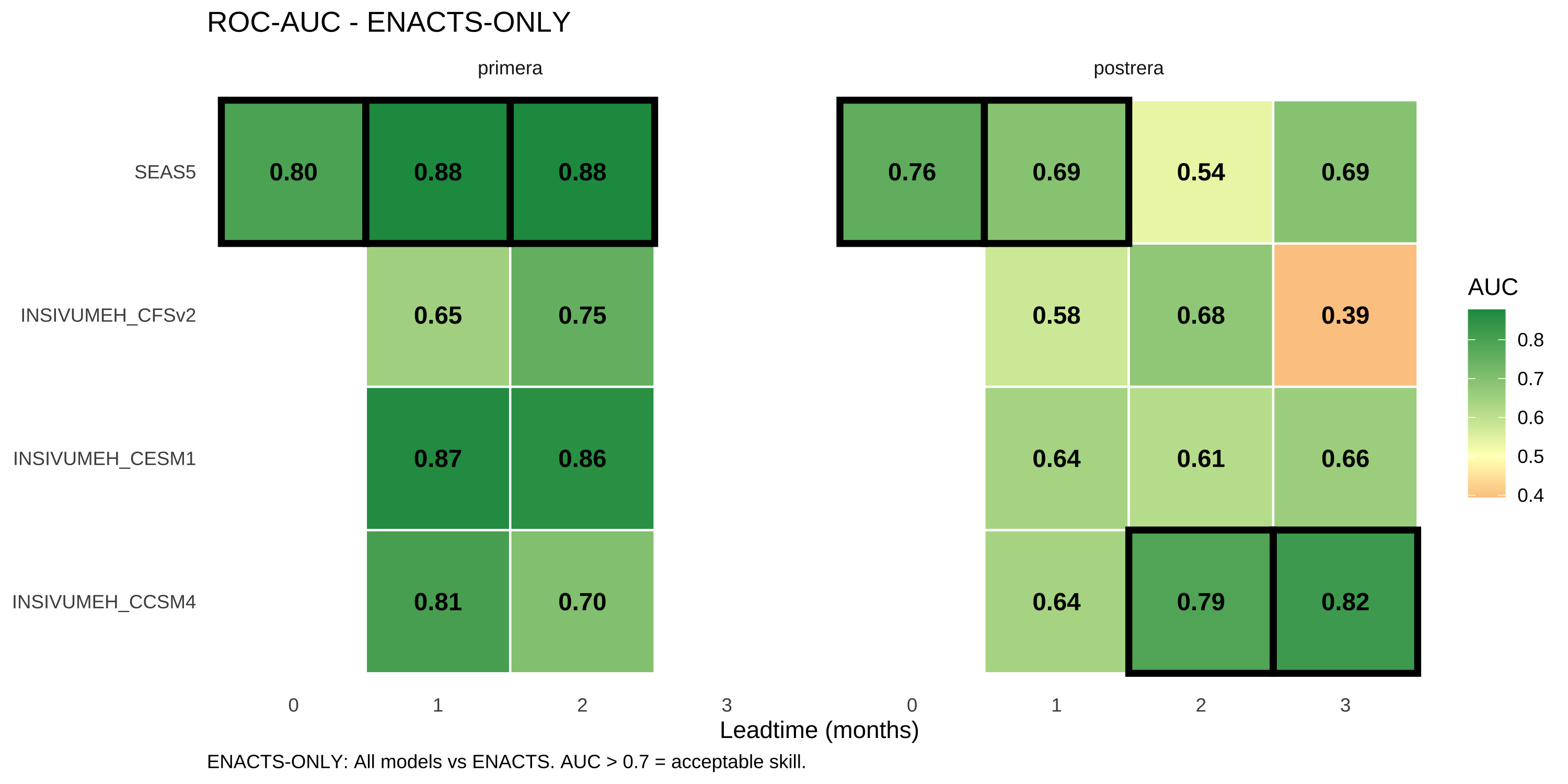
Of these, ROC-AUC is particularly interpretable for operational decisions. An AUC of 0.75 means: “If you randomly select a drought year and a non-drought year, there’s a 75% chance the forecast correctly identifies which is drier.” This directly answers whether the forecast can discriminate drought from non-drought conditions - the core operational question.

Setup: Libraries and data loading
library(tidyverse)
library(lubridate)
library(cumulus)
library(yardstick)
library(gghdx)
gghdx()

box::use(../../R/enacts)
box::use(../../R/seas5)

set.seed(42)

# Configuration
BASELINE_START <- 2000
BASELINE_END <- 2024
PRIMERA_MONTHS <- 5:8
POSTRERA_MONTHS <- 9:11
PRIMERA_ISSUED_MONTHS <- c(3, 4, 5)
POSTRERA_ISSUED_MONTHS <- c(6, 7, 8, 9)

# Helper function
calc_rp_threshold <- function(x, rp_target = 4, direction = -1) {
  x <- x[!is.na(x)]
  n <- length(x)
  if (n < 3) return(NA_real_)
  ranks <- rank(x * -direction, ties.method = "average")
  rp <- (n + 1) / ranks
  approx(rp, x, xout = rp_target, rule = 2)$y
}
Load forecast and observation data
# Load forecasts
df_insiv <- cumulus::blob_read(
  name = "ds-aa-lac-dry-corridor/data/processed/insivumeh_special/insivumeh_special_models_zonal_seasonal_chiquimula.parquet",
  container = "projects"
)
df_enacts <- enacts$load_enacts_seasonal("chiquimula")
df_seas5 <- seas5$load_seas5_seasonal()

# Load ERA5
con <- pg_con()
df_era5_raw <- tbl(con, "era5") |>
  filter(pcode == "GT20") |>
  collect() |>
  mutate(
    year = year(valid_date),
    month = month(valid_date),
    mean = mean * days_in_month(valid_date)
  )
DBI::dbDisconnect(con)

# Aggregate ERA5 to seasonal
aggregate_obs_seasonal <- function(df, window_name) {
  months <- if (window_name == "primera") PRIMERA_MONTHS else POSTRERA_MONTHS
  df |>
    filter(month %in% months) |>
    group_by(year) |>
    summarise(obs_mm = sum(value, na.rm = TRUE), .groups = "drop") |>
    mutate(window = window_name)
}

df_era5 <- bind_rows(
  aggregate_obs_seasonal(df_era5_raw |> rename(value = mean), "primera"),
  aggregate_obs_seasonal(df_era5_raw |> rename(value = mean), "postrera")
)

# Combine forecasts
df_fcst_all <- bind_rows(df_insiv, df_seas5) |>
  filter(year >= BASELINE_START, year <= BASELINE_END)

# Filter to operational leadtimes
df_fcst_filtered <- df_fcst_all |>
  mutate(issued_month = month(issued_date)) |>
  filter(
    (window == "primera" & issued_month %in% PRIMERA_ISSUED_MONTHS) |
    (window == "postrera" & issued_month %in% POSTRERA_ISSUED_MONTHS)
  )

3.2 Comparison Frameworks

NoteTwo Ways to Validate Forecasts

Native Comparison: Each model validated against its “natural” observation source

  • SEAS5 vs ERA5 (both from ECMWF)
  • INSIVUMEH vs ENACTS (regional data)

ENACTS-only: All models validated against ENACTS

  • Allows direct model-to-model comparison
  • ENACTS is the operational observation source

3.3 Method 1: Correlation Metrics

3.3.1 What It Measures

Correlation measures whether forecasts correctly identify which years are wetter or drier than average. A forecast doesn’t need to predict exact rainfall amounts - it just needs to rank years correctly.

3.3.2 Metrics

Metric Formula Interpretation
Spearman ρ Rank correlation Did wet years get higher forecasts? Robust to outliers.
Pearson r Linear correlation Same, but sensitive to extreme values.

3.3.3 Strengths & Weaknesses

Strengths

  • Measures interannual variability skill
  • No threshold dependence
  • Works on any units (mm or z-scores)
  • Spearman is robust to outliers

Weaknesses

  • Doesn’t measure absolute accuracy
  • A forecast could rank years perfectly but have huge bias
  • Sample size matters (n=25 years)
Calculate standardized anomalies
# Forecast anomalies
df_fcst_anom <- df_fcst_filtered |>
  group_by(forecast_source, window, leadtime) |>
  mutate(
    fcst_mean = mean(value, na.rm = TRUE),
    fcst_sd = sd(value, na.rm = TRUE),
    fcst_anom = (value - fcst_mean) / fcst_sd
  ) |>
  ungroup() |>
  select(year, window, leadtime, forecast_source, value, fcst_anom)

# Observation anomalies
calc_obs_anom <- function(df, obs_name) {
  df |>
    filter(year >= BASELINE_START, year <= BASELINE_END) |>
    group_by(window) |>
    mutate(
      obs_mean = mean(obs_mm, na.rm = TRUE),
      obs_sd = sd(obs_mm, na.rm = TRUE),
      obs_anom = (obs_mm - obs_mean) / obs_sd
    ) |>
    ungroup() |>
    mutate(obs_source = obs_name) |>
    select(year, window, obs_mm, obs_anom, obs_source)
}

df_enacts_anom <- calc_obs_anom(df_enacts, "ENACTS")
df_era5_anom <- calc_obs_anom(df_era5, "ERA5")

# Join - Native
df_anom_native <- bind_rows(
  df_fcst_anom |> filter(forecast_source == "SEAS5") |>
    inner_join(df_era5_anom, by = c("year", "window")),
  df_fcst_anom |> filter(str_detect(forecast_source, "INSIVUMEH")) |>
    inner_join(df_enacts_anom, by = c("year", "window"))
)

# Join - ENACTS-only
df_anom_enacts <- df_fcst_anom |>
  inner_join(df_enacts_anom, by = c("year", "window"))
Calculate continuous metrics
calc_continuous_metrics <- function(df) {
  df |>
    group_by(forecast_source, window, leadtime, obs_source) |>
    summarise(
      n = n(),
      spearman = cor(fcst_anom, obs_anom, method = "spearman", use = "complete.obs"),
      pearson = cor(fcst_anom, obs_anom, method = "pearson", use = "complete.obs"),
      rmse = sqrt(mean((fcst_anom - obs_anom)^2, na.rm = TRUE)),
      mae = mean(abs(fcst_anom - obs_anom), na.rm = TRUE),
      bias_mm = mean(value - obs_mm, na.rm = TRUE),
      .groups = "drop"
    )
}

df_metrics_native <- calc_continuous_metrics(df_anom_native)
df_metrics_enacts <- calc_continuous_metrics(df_anom_enacts)

3.3.4 Results: Spearman Correlation

Heatmap function
create_metric_heatmap <- function(df, metric_col, metric_name, title, caption,
                                  midpoint = 0, lower_is_better = FALSE) {
  df_plot <- df |>
    filter(!is.na(!!sym(metric_col))) |>
    mutate(window = factor(window, levels = c("primera", "postrera"))) |>
    group_by(window, leadtime) |>
    mutate(is_best = if (lower_is_better) {
      !!sym(metric_col) == min(!!sym(metric_col), na.rm = TRUE)
    } else {
      !!sym(metric_col) == max(!!sym(metric_col), na.rm = TRUE)
    }) |>
    ungroup()

  ggplot(df_plot, aes(x = factor(leadtime), y = forecast_source)) +
    geom_tile(aes(fill = !!sym(metric_col)), color = "white", linewidth = 0.5) +
    geom_tile(
      data = df_plot |> filter(is_best),
      fill = NA, color = "black", linewidth = 1.5
    ) +
    geom_text(aes(label = sprintf("%.2f", !!sym(metric_col))), size = 4, fontface = "bold", color = "black") +
    facet_wrap(~window) +
    scale_fill_gradient2(
      low = "#D73027", mid = "#FFFFBF", high = "#1A9850",
      midpoint = midpoint, name = metric_name
    ) +
    labs(title = title, x = "Leadtime (months)", y = NULL, caption = caption) +
    theme_minimal() +
    theme(legend.position = "right", panel.grid = element_blank(),
          plot.caption = element_text(hjust = 0))
}
Code
create_metric_heatmap(
  df_metrics_native, "spearman", "Spearman ρ",
  "Spearman Rank Correlation - NATIVE",
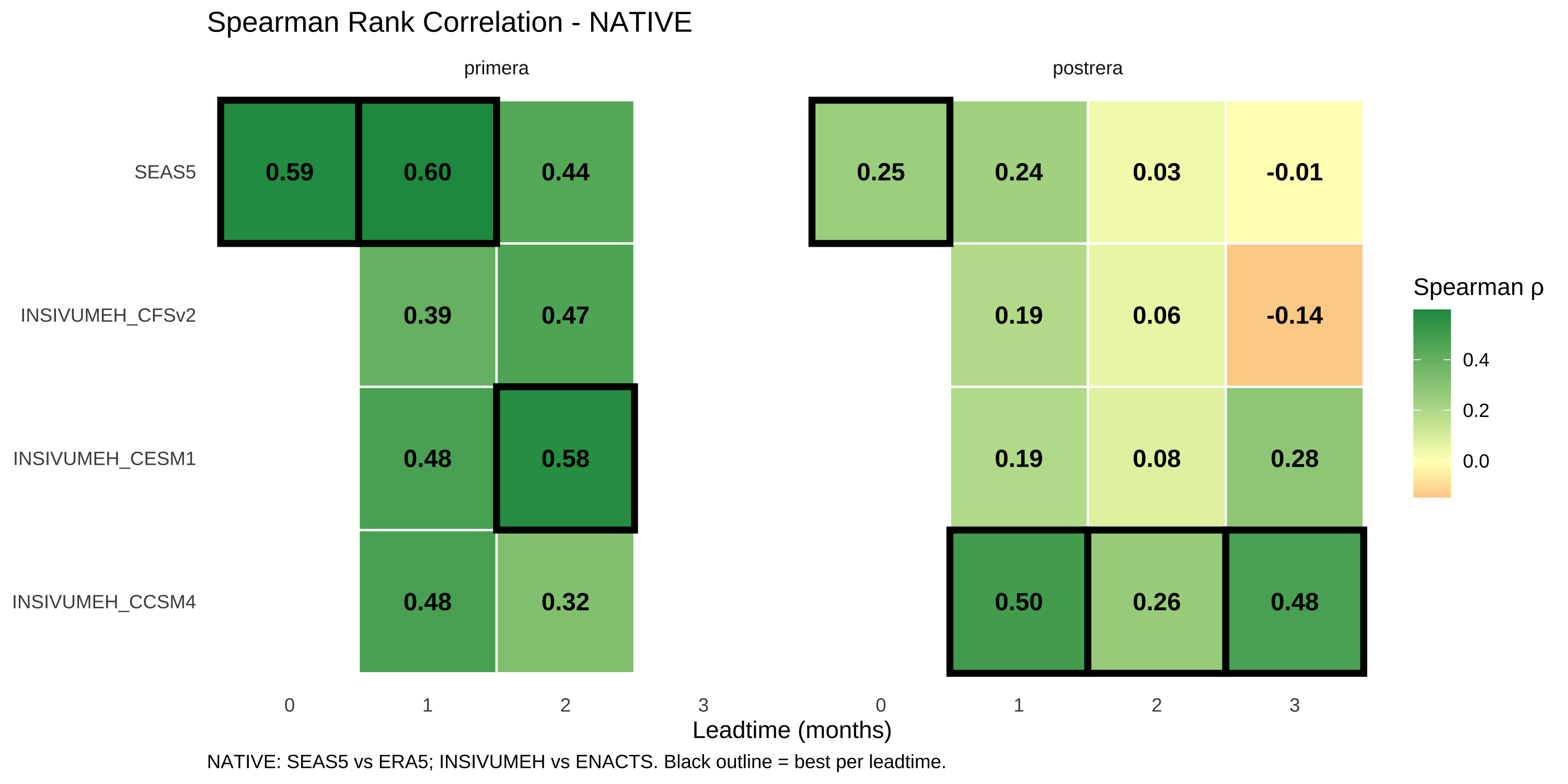
  "NATIVE: SEAS5 vs ERA5; INSIVUMEH vs ENACTS. Black outline = best per leadtime."
)

Code
create_metric_heatmap(
  df_metrics_enacts, "spearman", "Spearman ρ",
  "Spearman Rank Correlation - ENACTS-ONLY",
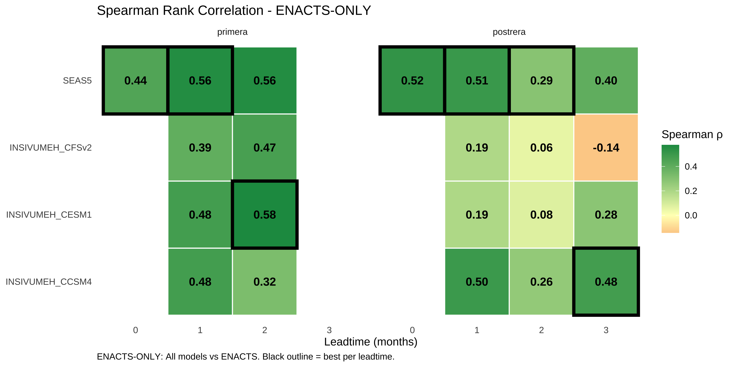
  "ENACTS-ONLY: All models vs ENACTS. Black outline = best per leadtime."
)

3.3.5 Interpretation: Correlation

TipKey Findings

Primera (May-Aug)

  • SEAS5 shows strong correlation (ρ = 0.56-0.60 at LT0-2)
  • INSIVUMEH models competitive at LT2, especially CESM1 (ρ = 0.58)
  • All models beat random (ρ = 0 expected by chance)

Postrera (Sep-Nov)

  • Weaker correlations across all models (ρ = 0.2-0.5)
  • SEAS5 slightly better at LT1 (ρ = 0.51)
  • CCSM4 shows unexpected strength at LT3 (ρ = 0.48)
  • More variability between leadtimes - less reliable signal

3.4 Method 2: Error Magnitude (RMSE, MAE)

3.4.1 What It Measures

Root Mean Square Error (RMSE) and Mean Absolute Error (MAE) measure how far forecasts deviate from observations in standardized units.

3.4.2 Metrics

Metric Formula Interpretation
RMSE √(mean((fcst - obs)²)) Penalizes large errors more heavily
MAE mean(|fcst - obs|) Equal penalty per unit error

3.4.3 Strengths & Weaknesses

Strengths

  • Measures absolute accuracy
  • RMSE sensitive to outliers (useful for flagging catastrophic misses)
  • MAE more robust, easier to interpret

Weaknesses

  • Depends on units (z-scores vs mm)
  • Can be dominated by a few bad years
  • Doesn’t distinguish bias from random error

3.4.4 Results: RMSE

Code
create_metric_heatmap(
  df_metrics_native, "rmse", "RMSE",
  "RMSE (Standardized Anomalies) - NATIVE",
  "NATIVE: SEAS5 vs ERA5; INSIVUMEH vs ENACTS. Lower = better. Black outline = best.",
  midpoint = 1, lower_is_better = TRUE
) +
  scale_fill_gradient2(low = "#1A9850", mid = "#FFFFBF", high = "#D73027",
                       midpoint = 1, name = "RMSE", limits = c(0.5, 1.5))

Code
create_metric_heatmap(
  df_metrics_enacts, "rmse", "RMSE",
  "RMSE (Standardized Anomalies) - ENACTS-ONLY",
  "ENACTS-ONLY: All models vs ENACTS. Lower = better. Black outline = best.",
  midpoint = 1, lower_is_better = TRUE
) +
  scale_fill_gradient2(low = "#1A9850", mid = "#FFFFBF", high = "#D73027",
                       midpoint = 1, name = "RMSE", limits = c(0.5, 1.5))

3.4.5 Interpretation: RMSE

TipKey Findings
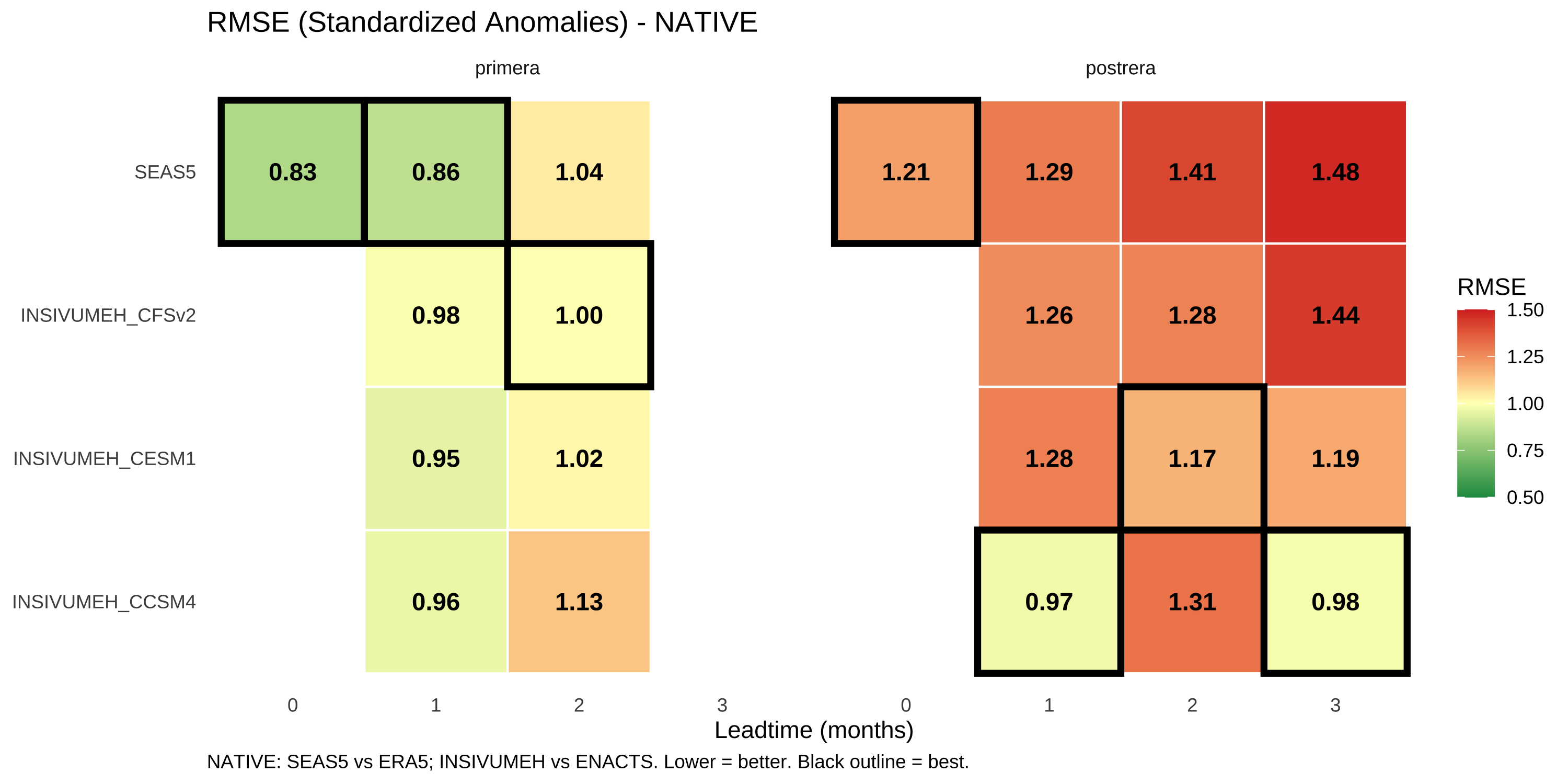
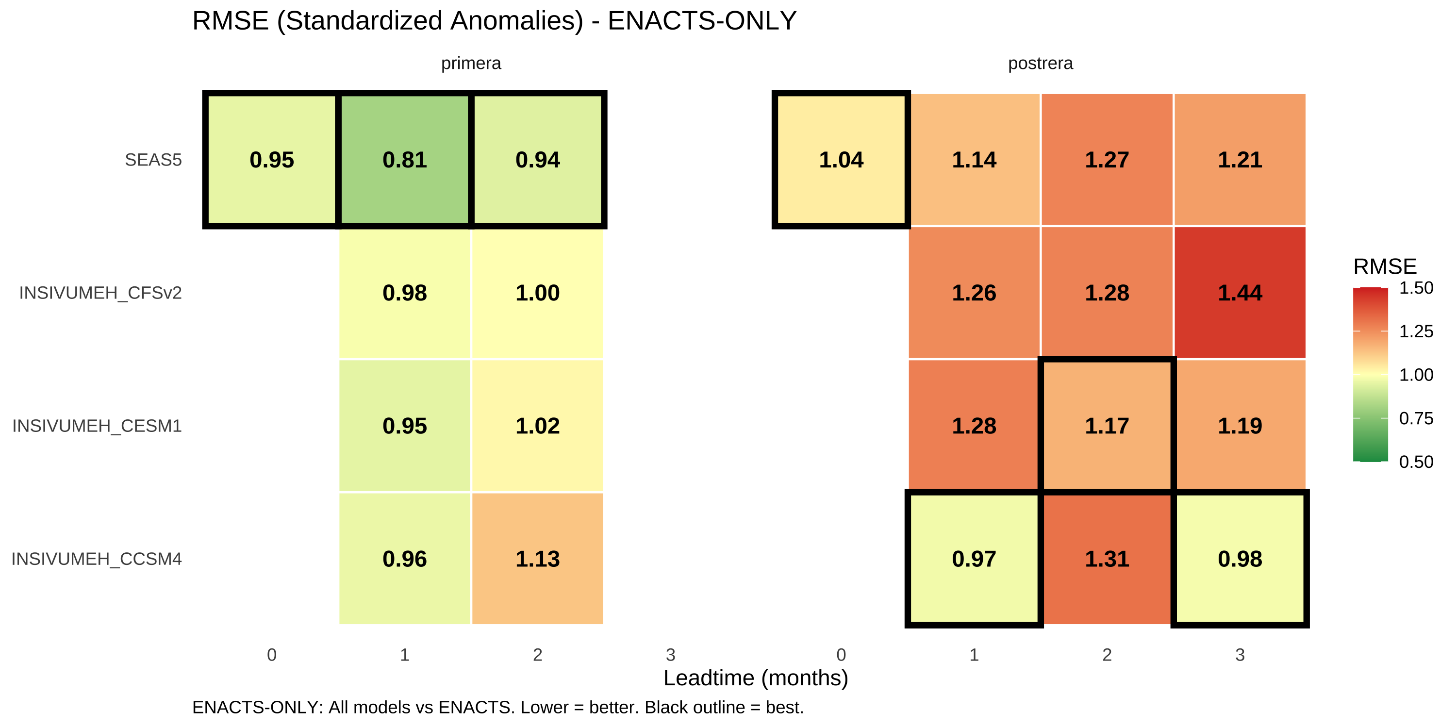
  • SEAS5 has lowest RMSE for Primera (0.81-0.95 vs 0.95-1.13 for INSIVUMEH)
  • For Postrera, CCSM4 often has lower RMSE than SEAS5
  • RMSE > 1.0 means error exceeds one standard deviation - forecasts add noise rather than signal
  • CFSv2 Postrera LT3 has RMSE = 1.44 - actively harmful predictions

3.5 Method 3: Bias

3.5.1 What It Measures

Bias measures systematic over- or under-prediction. A forecast with zero bias is “calibrated” on average, even if individual predictions are wrong.

3.5.2 Formula

\[\text{Bias} = \text{mean}(\text{forecast} - \text{observed})\]

  • Positive bias: Forecast too wet
  • Negative bias: Forecast too dry

3.5.3 Strengths & Weaknesses

Strengths

  • Easy to interpret (in mm)
  • Can be corrected with simple adjustments
  • Reveals systematic model issues

Weaknesses

  • Hides random error (a model can have zero bias but huge scatter)
  • Must use raw mm, not z-scores (z-score bias is always ~0 by construction)
WarningImportant Note on Units

Bias must be calculated on raw millimeters, not standardized anomalies. When you standardize to z-scores, you force the mean to zero - so bias between two z-scored series is mathematically guaranteed to be ~0, which is meaningless.

3.5.4 Results: Bias (Raw mm)

Bias heatmap function
create_bias_heatmap <- function(df, title, caption) {
  df_plot <- df |>
    filter(!is.na(bias_mm)) |>
    mutate(window = factor(window, levels = c("primera", "postrera"))) |>
    group_by(window, leadtime) |>
    mutate(is_best = abs(bias_mm) == min(abs(bias_mm), na.rm = TRUE)) |>
    ungroup()

  bias_max <- max(abs(df_plot$bias_mm), na.rm = TRUE)

  ggplot(df_plot, aes(x = factor(leadtime), y = forecast_source)) +
    geom_tile(aes(fill = bias_mm), color = "white", linewidth = 0.5) +
    geom_tile(
      data = df_plot |> filter(is_best),
      fill = NA, color = "black", linewidth = 1.5
    ) +
    geom_text(aes(label = sprintf("%.0f", bias_mm)), size = 4, fontface = "bold", color = "black") +
    facet_wrap(~window) +
    scale_fill_gradient2(
      low = "#D73027", mid = "#FFFFBF", high = "#1A9850",
      midpoint = 0, limits = c(-bias_max, bias_max), name = "Bias (mm)"
    ) +
    labs(title = title, x = "Leadtime (months)", y = NULL, caption = caption) +
    theme_minimal() +
    theme(legend.position = "right", panel.grid = element_blank(),
          plot.caption = element_text(hjust = 0))
}
Code
create_bias_heatmap(
  df_metrics_native,
  "Mean Bias - NATIVE",
  "NATIVE: SEAS5 vs ERA5; INSIVUMEH vs ENACTS. Units: mm. Black outline = closest to zero."
)

Code
create_bias_heatmap(
  df_metrics_enacts,
  "Mean Bias - ENACTS-ONLY",
  "ENACTS-ONLY: All models vs ENACTS. Units: mm. Black outline = closest to zero."
)

3.5.5 Interpretation: Bias

TipKey Findings

Primera

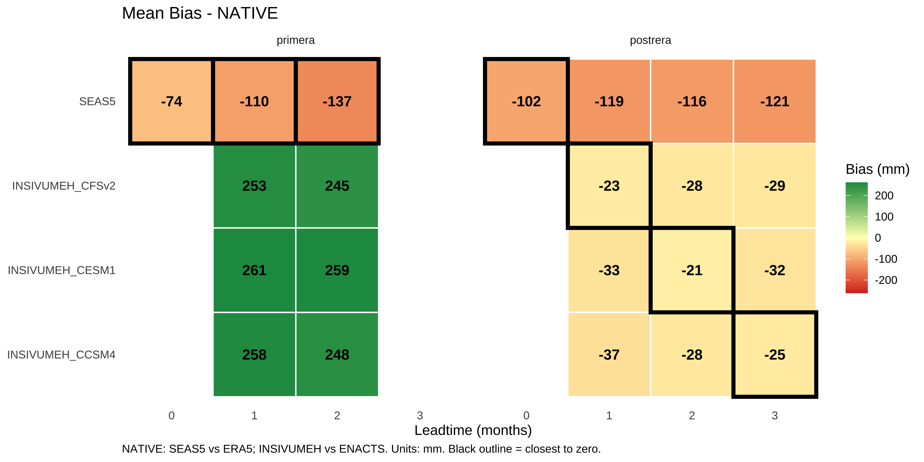
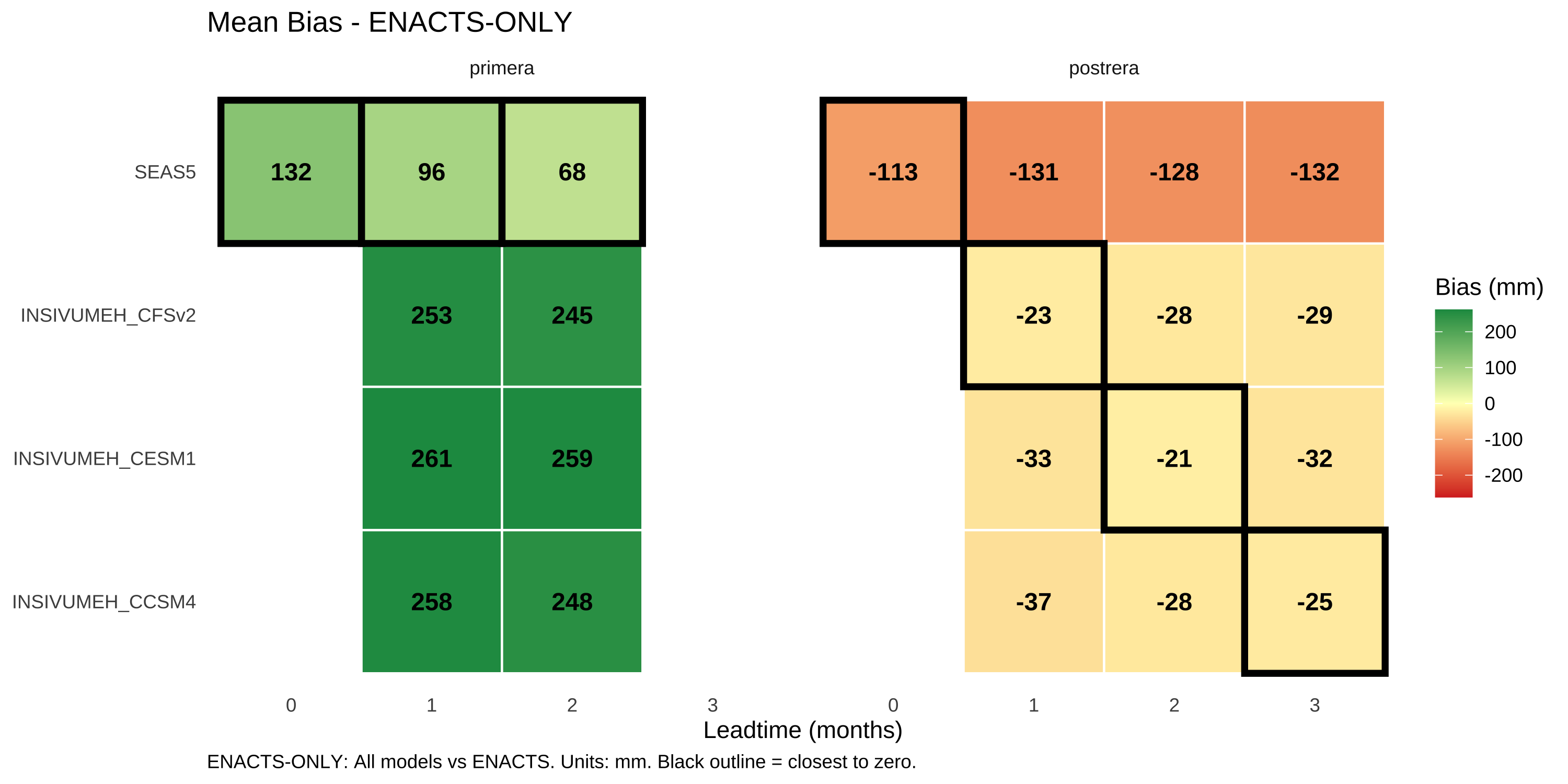
  • All models are biased wet (positive bias)
  • SEAS5: +68 to +132mm too wet
  • INSIVUMEH models: +244 to +262mm too wet (severe overestimation)
  • This means forecasts systematically predict more rain than actually falls

Postrera

  • All models are biased dry (negative bias)
  • SEAS5: -113 to -132mm too dry
  • INSIVUMEH models: -21 to -37mm too dry (much smaller bias)
  • For Postrera, INSIVUMEH has better calibration than SEAS5

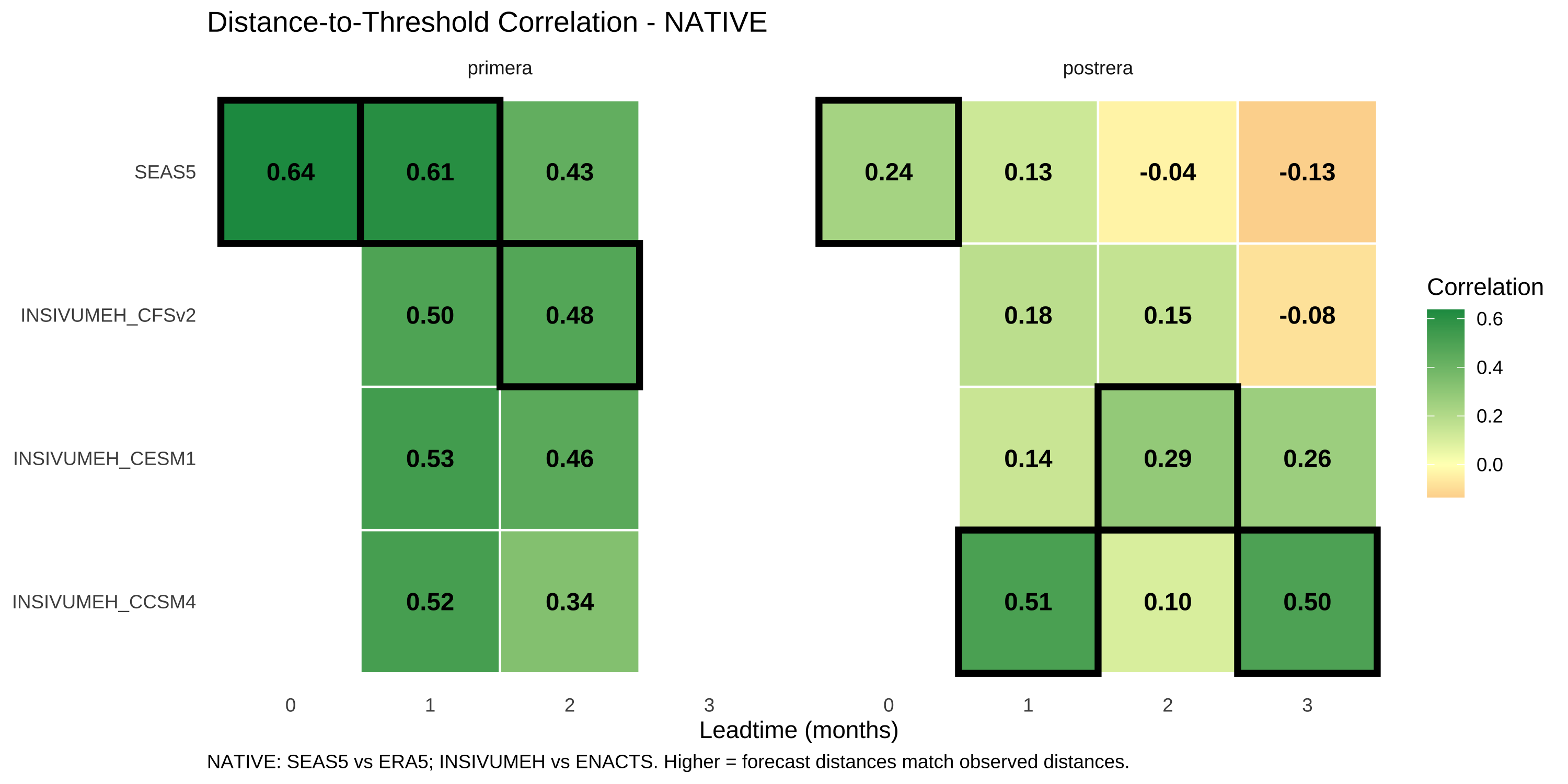
3.6 Method 4: Distance-to-Threshold

3.6.1 What It Measures

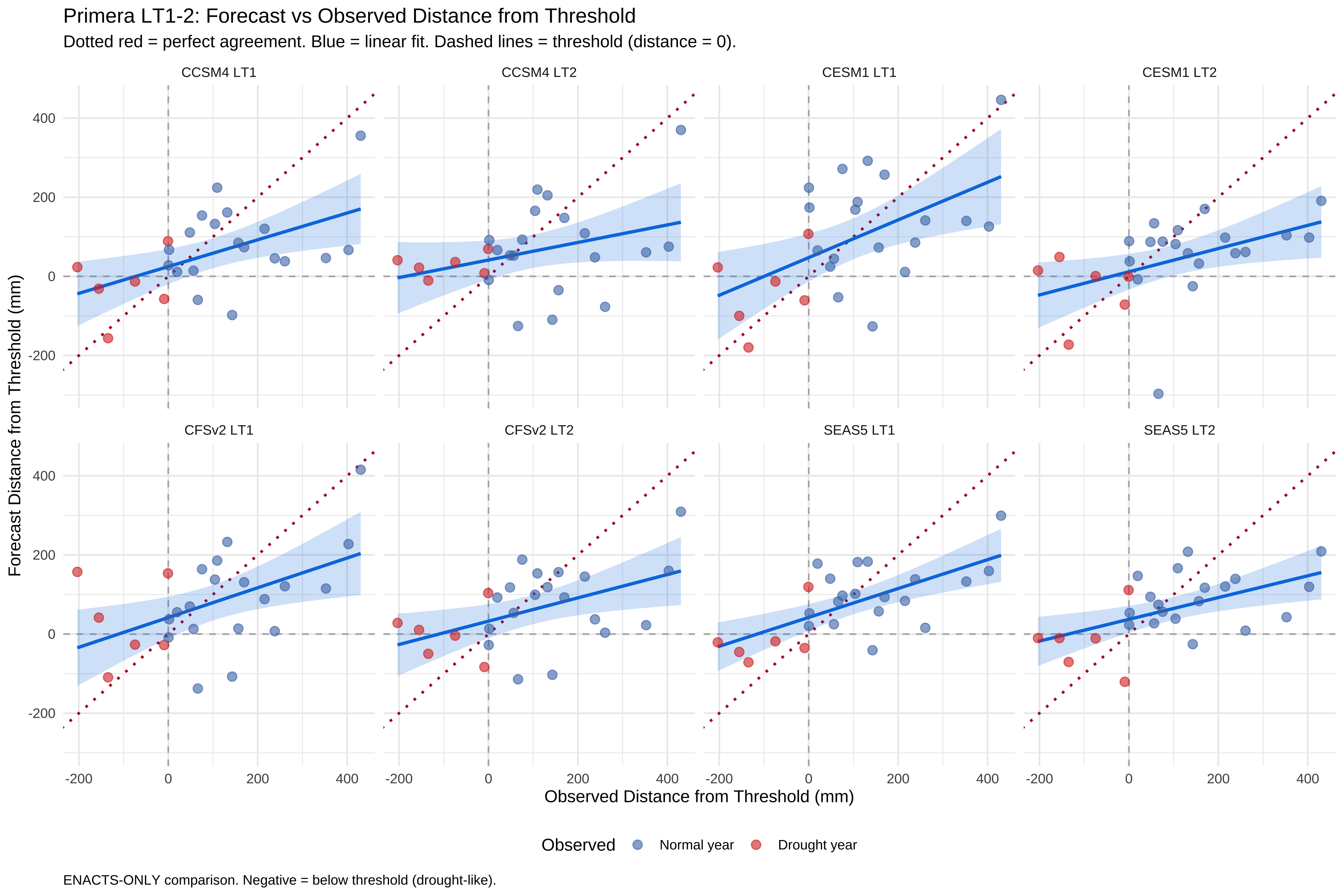
Instead of binary hit/miss, measure how far each forecast and observation was from their respective drought thresholds. Then correlate these distances.

3.6.2 Why This Matters

Consider two “false positive” cases:

  1. Forecast: 10mm below threshold. Observed: 5mm above threshold. (Near miss)
  2. Forecast: 100mm below threshold. Observed: 150mm above threshold. (Confident and wrong)

Binary metrics score both as equally wrong. Distance-to-threshold reveals that Case 1 was almost right, while Case 2 was a confident failure.

3.6.3 Calculation

fcst_distance = forecast_value - forecast_threshold
obs_distance = observed_value - observed_threshold

distance_correlation = cor(fcst_distance, obs_distance)
  • Negative distance = below threshold (drought-like)
  • Positive distance = above threshold (normal)

3.6.4 Strengths & Weaknesses

Strengths

  • Gives partial credit for near-misses
  • Operationally relevant (close calls matter)
  • Uses actual mm, not abstract scores

Weaknesses

  • Still depends on threshold choice
  • Correlation can be high even if absolute distances don’t match
Calculate distance-to-threshold
# Observation thresholds
obs_thresh_enacts <- df_enacts |>
  filter(year >= BASELINE_START, year <= BASELINE_END) |>
  group_by(window) |>
  summarise(obs_thresh = calc_rp_threshold(obs_mm, 4, -1), .groups = "drop")

obs_thresh_era5 <- df_era5 |>
  filter(year >= BASELINE_START, year <= BASELINE_END) |>
  group_by(window) |>
  summarise(obs_thresh = calc_rp_threshold(obs_mm, 4, -1), .groups = "drop")

# Forecast thresholds
fcst_thresholds <- df_fcst_filtered |>
  group_by(forecast_source, window, leadtime) |>
  summarise(fcst_thresh = calc_rp_threshold(value, 4, -1), .groups = "drop")

# Build distance data
build_distance_data <- function(df_fcst, df_obs, obs_thresholds, obs_name) {
  df_obs_filtered <- df_obs |> filter(year >= BASELINE_START, year <= BASELINE_END)

  df_fcst |>
    left_join(df_obs_filtered |> select(year, window, obs_mm), by = c("year", "window")) |>
    left_join(obs_thresholds, by = "window") |>
    left_join(fcst_thresholds, by = c("forecast_source", "window", "leadtime")) |>
    mutate(
      fcst_distance_mm = value - fcst_thresh,
      obs_distance_mm = obs_mm - obs_thresh,
      fcst_drought = value <= fcst_thresh,
      obs_drought = obs_mm <= obs_thresh,
      obs_source = obs_name
    ) |>
    filter(!is.na(obs_mm), !is.na(fcst_thresh))
}

df_dist_native <- bind_rows(
  build_distance_data(df_fcst_filtered |> filter(forecast_source == "SEAS5"),
                      df_era5, obs_thresh_era5, "ERA5"),
  build_distance_data(df_fcst_filtered |> filter(str_detect(forecast_source, "INSIVUMEH")),
                      df_enacts, obs_thresh_enacts, "ENACTS")
)

df_dist_enacts <- build_distance_data(df_fcst_filtered, df_enacts, obs_thresh_enacts, "ENACTS")

# Calculate distance metrics
calc_distance_metrics <- function(df) {
  df |>
    group_by(forecast_source, window, leadtime, obs_source) |>
    summarise(
      dist_corr = cor(fcst_distance_mm, obs_distance_mm, use = "complete.obs"),
      mae_dist = mean(abs(fcst_distance_mm - obs_distance_mm), na.rm = TRUE),
      .groups = "drop"
    )
}

df_dist_metrics_native <- calc_distance_metrics(df_dist_native)
df_dist_metrics_enacts <- calc_distance_metrics(df_dist_enacts)

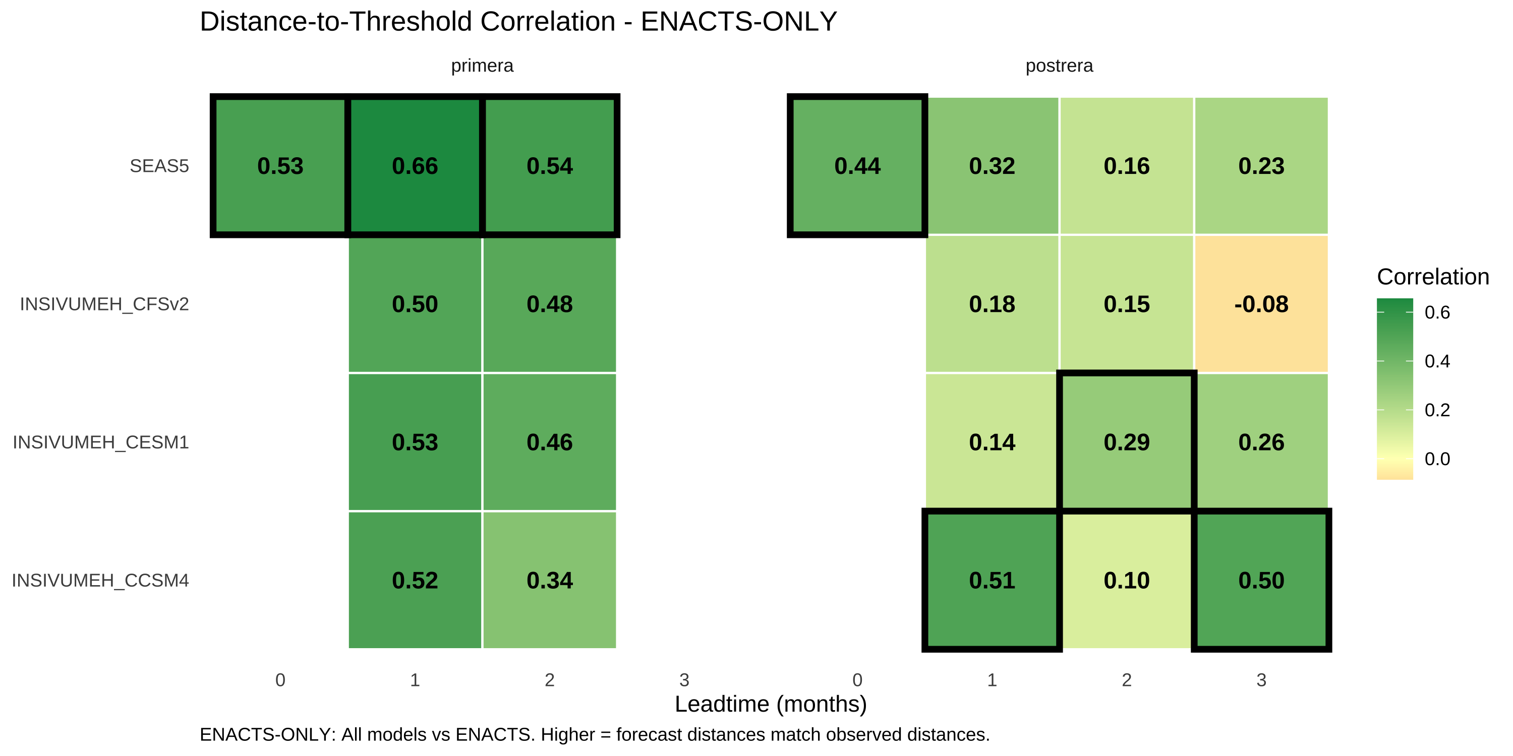
3.6.5 Results: Distance Correlation

Code
create_metric_heatmap(
  df_dist_metrics_native, "dist_corr", "Correlation",
  "Distance-to-Threshold Correlation - NATIVE",
  "NATIVE: SEAS5 vs ERA5; INSIVUMEH vs ENACTS. Higher = forecast distances match observed distances."
)

Code
create_metric_heatmap(
  df_dist_metrics_enacts, "dist_corr", "Correlation",
  "Distance-to-Threshold Correlation - ENACTS-ONLY",
  "ENACTS-ONLY: All models vs ENACTS. Higher = forecast distances match observed distances."
)

3.6.6 Scatter Plot: Distance Comparison

Distance scatter plots
df_dist_enacts |>
  filter(window == "primera", leadtime %in% c(1, 2)) |>
  mutate(
    model = str_remove(forecast_source, "INSIVUMEH_"),
    facet = paste0(model, " LT", leadtime)
  ) |>
  ggplot(aes(x = obs_distance_mm, y = fcst_distance_mm)) +
  geom_hline(yintercept = 0, color = "grey70", linetype = "dashed") +
  geom_vline(xintercept = 0, color = "grey70", linetype = "dashed") +
  geom_abline(slope = 1, intercept = 0, color = "#B2182B", linetype = "dotted", linewidth = 0.8) +
  geom_smooth(method = "lm", se = TRUE, color = "#007CE1", fill = "#007CE1", alpha = 0.2) +
  geom_point(aes(color = obs_drought), alpha = 0.6, size = 2.5) +
  facet_wrap(~facet, ncol = 4) +
  scale_color_manual(
    values = c("TRUE" = "#D73027", "FALSE" = "#4575B4"),
    labels = c("TRUE" = "Drought year", "FALSE" = "Normal year"),
    name = "Observed"
  ) +
  labs(
    title = "Primera LT1-2: Forecast vs Observed Distance from Threshold",
    subtitle = "Dotted red = perfect agreement. Blue = linear fit. Dashed lines = threshold (distance = 0).",
    x = "Observed Distance from Threshold (mm)",
    y = "Forecast Distance from Threshold (mm)",
    caption = "ENACTS-ONLY comparison. Negative = below threshold (drought-like)."
  ) +
  theme_minimal() +
  theme(legend.position = "bottom", plot.caption = element_text(hjust = 0))

3.6.7 Interpretation: Distance-to-Threshold

TipKey Findings

Primera

  • SEAS5 LT1 has the strongest distance correlation (r = 0.66)
  • When SEAS5 says “drier than usual”, observations tend to agree
  • INSIVUMEH models also show skill (r = 0.5-0.53)

Postrera

  • CCSM4 shows best distance skill at LT1 (r = 0.51)
  • SEAS5 Postrera distance correlation drops sharply at LT2 (r = 0.16)
  • CFSv2 LT3 has negative correlation (r = -0.08) - actively misleading

3.7 Method 5: ROC Curves & AUC

3.7.1 What It Measures

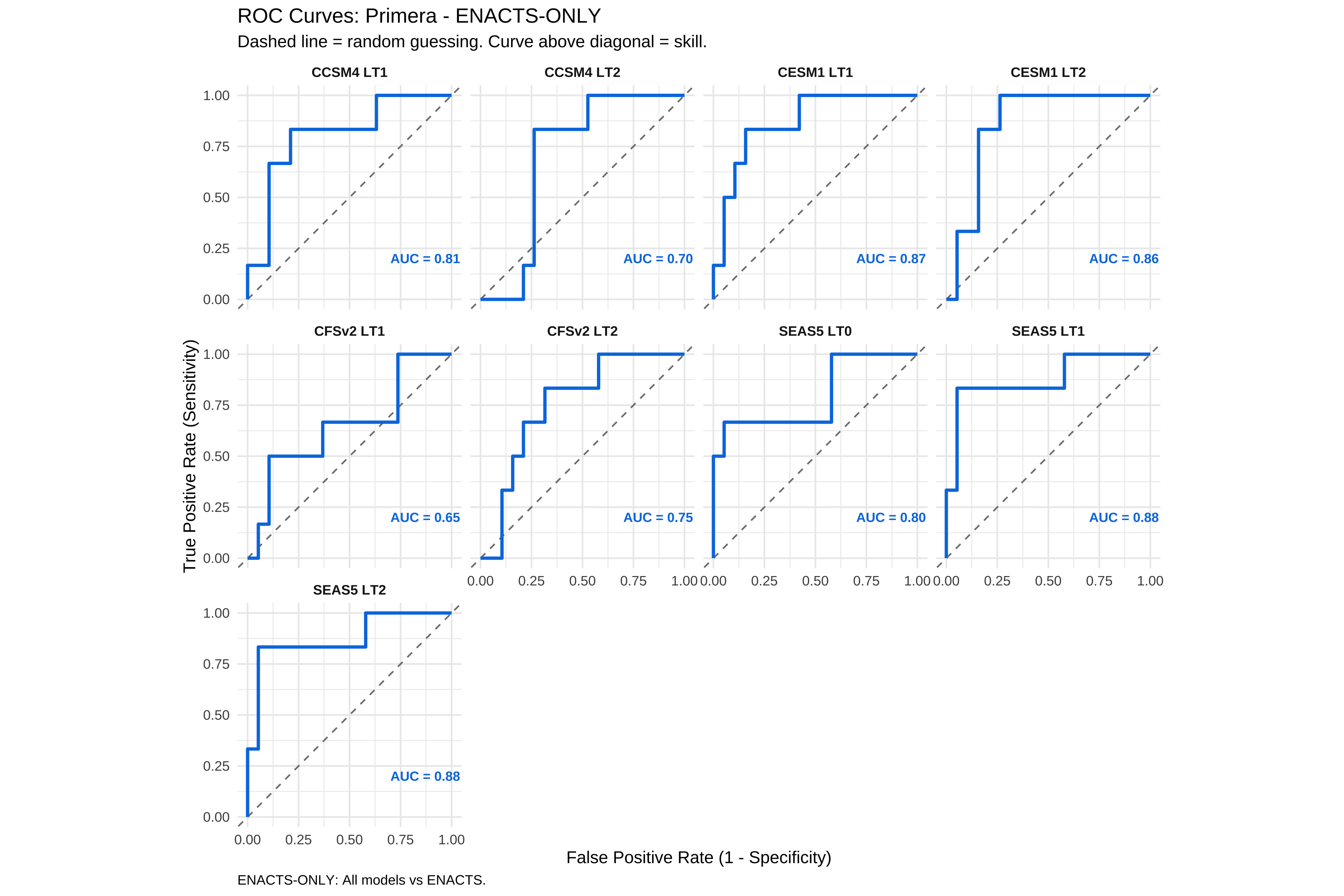
ROC (Receiver Operating Characteristic) curves measure ranking skill: did lower forecast values correspond to actual drought years?

Unlike binary metrics, ROC doesn’t require choosing a specific threshold. It asks: “If I ranked all years by forecast value, would drought years tend to be at the bottom?”

3.7.2 How to Read an ROC Curve

  • Diagonal line: Random guessing (AUC = 0.5)
  • Curve above diagonal: Skill (drought years get lower forecasts)
  • Curve below diagonal: Inverted skill (drought years get higher forecasts - very bad)

3.7.3 AUC Interpretation

AUC Interpretation
0.9-1.0 Outstanding
0.8-0.9 Excellent
0.7-0.8 Acceptable
0.5-0.7 Poor
< 0.5 Worse than random

3.7.4 Strengths & Weaknesses

Strengths

  • Threshold-independent
  • Measures ranking/discrimination skill
  • Well-understood statistically

Weaknesses

  • Doesn’t measure calibration
  • Can be high even with severe bias
  • Small sample size (6 drought years) limits precision
Calculate ROC and AUC
# Build ROC data
build_roc_data <- function(df_fcst, df_obs, obs_thresholds, obs_name) {
  df_obs_filtered <- df_obs |> filter(year >= BASELINE_START, year <= BASELINE_END)

  df_fcst |>
    left_join(df_obs_filtered |> select(year, window, obs_mm), by = c("year", "window")) |>
    left_join(obs_thresholds, by = "window") |>
    mutate(
      truth = factor(obs_mm <= obs_thresh, c(TRUE, FALSE), c("drought", "no_drought")),
      drought_score = -value,  # Lower forecast = higher drought score
      obs_source = obs_name
    ) |>
    filter(!is.na(truth))
}

df_roc_native <- bind_rows(
  build_roc_data(df_fcst_filtered |> filter(forecast_source == "SEAS5"),
                 df_era5, obs_thresh_era5, "ERA5"),
  build_roc_data(df_fcst_filtered |> filter(str_detect(forecast_source, "INSIVUMEH")),
                 df_enacts, obs_thresh_enacts, "ENACTS")
)

df_roc_enacts <- build_roc_data(df_fcst_filtered, df_enacts, obs_thresh_enacts, "ENACTS")

# Calculate AUC
calc_auc <- function(df) {
  if (length(unique(df$truth)) < 2) return(NA_real_)
  roc_auc(df, truth = truth, drought_score, event_level = "first")$.estimate
}

df_auc_native <- df_roc_native |>
  group_by(forecast_source, window, leadtime, obs_source) |>
  summarise(auc = calc_auc(pick(everything())), .groups = "drop")

df_auc_enacts <- df_roc_enacts |>
  group_by(forecast_source, window, leadtime) |>
  summarise(auc = calc_auc(pick(everything())), obs_source = "ENACTS", .groups = "drop")

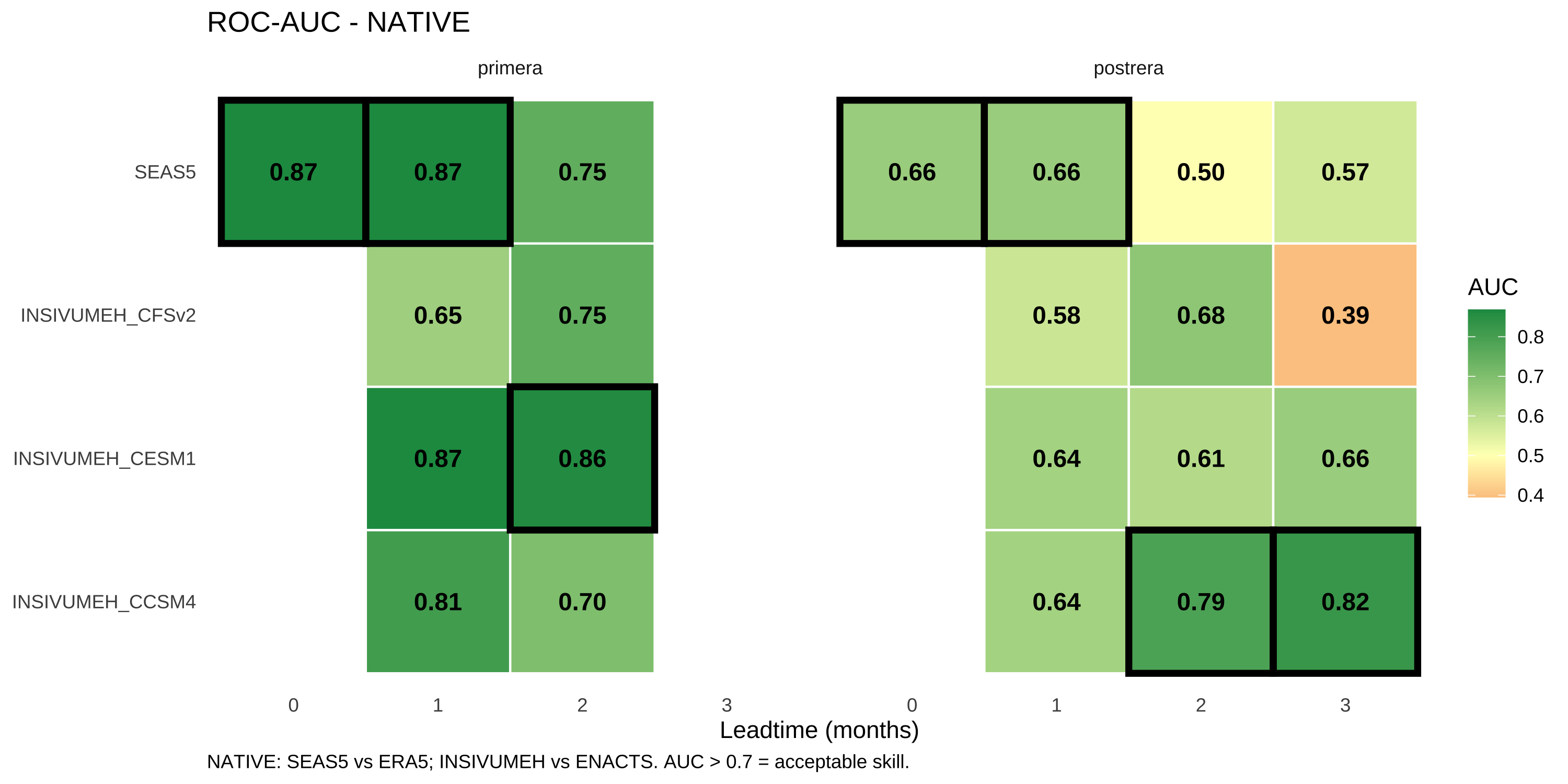
3.7.5 Results: AUC Heatmaps

Code
create_metric_heatmap(
  df_auc_native, "auc", "AUC",
  "ROC-AUC - NATIVE",
  "NATIVE: SEAS5 vs ERA5; INSIVUMEH vs ENACTS. AUC > 0.7 = acceptable skill.",
  midpoint = 0.5
)

Code
create_metric_heatmap(
  df_auc_enacts, "auc", "AUC",
  "ROC-AUC - ENACTS-ONLY",
  "ENACTS-ONLY: All models vs ENACTS. AUC > 0.7 = acceptable skill.",
  midpoint = 0.5
)

3.7.6 ROC Curves: Primera

ROC curves
# Calculate ROC curves
calc_roc_curve <- function(df) {
  if (length(unique(df$truth)) < 2) return(tibble(specificity = NA, sensitivity = NA))
  roc_curve(df, truth = truth, drought_score, event_level = "first")
}

df_roc_curves_enacts <- df_roc_enacts |>
  group_by(forecast_source, window, leadtime) |>
  group_modify(~calc_roc_curve(.x)) |>
  ungroup()

df_roc_curves_enacts |>
  filter(window == "primera", !is.na(specificity)) |>
  mutate(
    model = str_remove(forecast_source, "INSIVUMEH_"),
    facet = paste0(model, " LT", leadtime)
  ) |>
  left_join(
    df_auc_enacts |> filter(window == "primera") |>
      mutate(model = str_remove(forecast_source, "INSIVUMEH_"),
             facet = paste0(model, " LT", leadtime),
             label = paste0("AUC = ", sprintf("%.2f", auc))),
    by = c("forecast_source", "window", "leadtime", "facet", "model")
  ) |>
  ggplot(aes(x = 1 - specificity, y = sensitivity)) +
  geom_abline(slope = 1, intercept = 0, linetype = "dashed", color = "grey50") +
  geom_path(color = "#007CE1", linewidth = 1) +
  geom_text(aes(x = 0.7, y = 0.2, label = label), hjust = 0, size = 3, fontface = "bold",
            color = "#007CE1", check_overlap = TRUE) +
  facet_wrap(~facet, ncol = 4) +
  coord_equal() +
  labs(
    title = "ROC Curves: Primera - ENACTS-ONLY",
    subtitle = "Dashed line = random guessing. Curve above diagonal = skill.",
    x = "False Positive Rate (1 - Specificity)",
    y = "True Positive Rate (Sensitivity)",
    caption = "ENACTS-ONLY: All models vs ENACTS."
  ) +
  theme_minimal() +
  theme(strip.text = element_text(face = "bold"), plot.caption = element_text(hjust = 0))

3.7.7 Interpretation: ROC-AUC

TipKey Findings

Primera

  • SEAS5 and CESM1 show excellent discrimination (AUC = 0.87-0.88 at LT1-2)
  • CCSM4 also strong (AUC = 0.81 at LT1)
  • All models beat random guessing

Postrera

  • Much weaker AUC across all models (0.5-0.8 range)
  • CCSM4 LT3 surprisingly good (AUC = 0.83)
  • SEAS5 LT2 near random (AUC = 0.54)
  • CFSv2 LT3 inverted (AUC = 0.40) - lower forecasts correspond to wetter years

3.8 Summary: Which Model Wins?

Summary comparison
df_summary <- df_metrics_enacts |>
  left_join(df_dist_metrics_enacts, by = c("forecast_source", "window", "leadtime", "obs_source")) |>
  left_join(df_auc_enacts, by = c("forecast_source", "window", "leadtime", "obs_source")) |>
  filter(leadtime %in% c(1, 2)) |>
  mutate(model = str_remove(forecast_source, "INSIVUMEH_")) |>
  select(model, window, leadtime, spearman, rmse, bias_mm, dist_corr, auc) |>
  mutate(across(c(spearman, rmse, dist_corr, auc), ~round(.x, 2)),
         bias_mm = round(bias_mm, 0))

3.8.1 Primera (MJJA)

Code
df_summary |>
  filter(window == "primera") |>
  arrange(leadtime, desc(auc)) |>
  knitr::kable(
    col.names = c("Model", "Window", "LT", "Spearman", "RMSE", "Bias (mm)", "Dist Corr", "AUC"),
    caption = "Primera: All metrics at LT1-2 (ENACTS-only)"
  )
Primera: All metrics at LT1-2 (ENACTS-only)
Model Window LT Spearman RMSE Bias (mm) Dist Corr AUC
SEAS5 primera 1 0.56 0.81 96 0.66 0.88
CESM1 primera 1 0.48 0.95 261 0.53 0.87
CCSM4 primera 1 0.48 0.96 258 0.52 0.81
CFSv2 primera 1 0.39 0.98 253 0.50 0.65
SEAS5 primera 2 0.56 0.94 68 0.54 0.88
CESM1 primera 2 0.58 1.02 259 0.46 0.86
CFSv2 primera 2 0.47 1.00 245 0.48 0.75
CCSM4 primera 2 0.32 1.13 248 0.34 0.70
NotePrimera Recommendation: SEAS5
  • Highest AUC (0.88 at both LT1 and LT2)
  • Highest distance correlation (0.66 at LT1)
  • Lowest RMSE (0.81 at LT1)
  • Smallest bias (+68 to +96mm vs +244-262mm for INSIVUMEH)
  • CESM1 is competitive but has much larger bias

3.8.2 Postrera (SON)

Code
df_summary |>
  filter(window == "postrera") |>
  arrange(leadtime, desc(auc)) |>
  knitr::kable(
    col.names = c("Model", "Window", "LT", "Spearman", "RMSE", "Bias (mm)", "Dist Corr", "AUC"),
    caption = "Postrera: All metrics at LT1-2 (ENACTS-only)"
  )
Postrera: All metrics at LT1-2 (ENACTS-only)
Model Window LT Spearman RMSE Bias (mm) Dist Corr AUC
SEAS5 postrera 1 0.51 1.14 -131 0.32 0.69
CCSM4 postrera 1 0.50 0.97 -37 0.51 0.64
CESM1 postrera 1 0.19 1.28 -33 0.14 0.64
CFSv2 postrera 1 0.19 1.26 -23 0.18 0.58
CCSM4 postrera 2 0.26 1.31 -28 0.10 0.79
CFSv2 postrera 2 0.06 1.28 -28 0.15 0.68
CESM1 postrera 2 0.08 1.17 -21 0.29 0.61
SEAS5 postrera 2 0.29 1.27 -128 0.16 0.54
NotePostrera Recommendation: Ambiguous

No clear winner - different metrics favor different models:

Metric LT1 Winner LT2 Winner
Spearman SEAS5 (0.51) SEAS5 (0.29)
RMSE CCSM4 (0.97) CESM1 (1.17)
Bias CFSv2 (-23mm) CESM1 (-21mm)
Dist Corr CCSM4 (0.51) CESM1 (0.29)
AUC SEAS5 (0.69) CCSM4 (0.79)

If forced to choose one model: CCSM4 has the best average AUC and distance correlation, but no model shows strong, consistent skill.


3.9 Conclusions

3.9.1 Key Takeaways

  1. Primera has genuine forecast skill across multiple metrics. SEAS5 is the clear winner with AUC values around 0.80 - meaning 80% probability of correctly ranking a drought vs non-drought year.

  2. Postrera remains challenging - no model shows consistent, strong skill. AUC values hover near 0.5-0.6 (barely above random guessing). Consider supplementing with monitoring-based triggers.

  3. ROC-AUC provides the clearest picture - it directly answers “can this forecast discriminate drought?” without depending on threshold choices. Binary F1 scores can be variable with small samples; AUC is more stable.

  4. Bias matters operationally - INSIVUMEH models systematically over-predict Primera rainfall by ~250mm. This could be corrected with simple bias adjustment if these models are used.

  5. Correlation and AUC tell consistent stories - both favor SEAS5 for Primera, show weaker skill for Postrera. When multiple metrics agree, we can be more confident in the assessment.
3.9.2 Operational Recommendations

Season Recommended Model Confidence Notes
Primera LT0 SEAS5 High Only option for May activation
Primera LT1-2 SEAS5 High Best on all metrics
Postrera LT1-2 CCSM4 or SEAS5 Low Consider ensemble or monitoring triggers