Chapters 2 and 3 evaluated forecasts against two observation sources:
ERA5: Global reanalysis (SEAS5’s “native” validation)
ENACTS: Station-blended satellite product (operational standard for Guatemala)
These showed consistent results: SEAS5 performs well for Primera, all models struggle with Postrera. But what if both observation sources happen to favor SEAS5? To break potential ties and increase confidence, we introduce a third independent observation source: CHIRPS.
4.2 Observational Data Sets
This analysis uses three independent observation sources:
CHIRPS (Climate Hazards Group InfraRed Precipitation with Station data) is a quasi-global rainfall dataset that blends satellite imagery with station data. Key characteristics:
Feature
CHIRPS
ENACTS
ERA5
Resolution
0.05° (~5km)
0.05° (~5km)
0.25° (~25km)
Source
Satellite + stations
Satellite + stations
Model reanalysis
Coverage
50°S-50°N
Regional
Global
Temporal
1981-present
Varies
1940-present
CHIRPS and ENACTS both blend satellite and station data, but use different algorithms and station networks. This makes CHIRPS a useful independent check - if forecasts perform well against multiple observation sources, we can be more confident in the skill assessment.
# Load forecastsdf_insiv <- cumulus::blob_read(name ="ds-aa-lac-dry-corridor/data/processed/insivumeh_special/insivumeh_special_models_zonal_seasonal_chiquimula.parquet",container ="projects")df_seas5 <- seas5$load_seas5_seasonal()# Load CHIRPS - extracted via GEE scriptdf_chirps_raw <- cumulus::blob_read(name ="ds-aa-lac-dry-corridor/raw/chirps/2026_cadc_drought_v3_aoi_chirps_monthly_historical.parquet",container ="projects")# Wrangle CHIRPS to seasonal totalsdf_chirps <- df_chirps_raw |>filter(ADM1_NAME =="Chiquimula") |>mutate(year =year(date),month =month(date),window =case_when( month %in% PRIMERA_MONTHS ~"primera", month %in% POSTRERA_MONTHS ~"postrera",TRUE~NA_character_ ) ) |>filter(!is.na(window), year >= BASELINE_START, year <= BASELINE_END) |>group_by(year, window) |>summarise(obs_mm =sum(value, na.rm =TRUE), .groups ="drop")# Combine forecastsdf_fcst_all <-bind_rows(df_insiv, df_seas5) |>filter(year >= BASELINE_START, year <= BASELINE_END)# Filter to operational leadtimesdf_fcst_filtered <- df_fcst_all |>mutate(issued_month =month(issued_date)) |>filter( (window =="primera"& issued_month %in% PRIMERA_ISSUED_MONTHS) | (window =="postrera"& issued_month %in% POSTRERA_ISSUED_MONTHS) )# Join forecasts with CHIRPSdf_joined <- df_fcst_filtered |>left_join(df_chirps, by =c("year", "window")) |>filter(!is.na(obs_mm)) # there are not any NA - any ways
4.3 Metrics Against CHIRPS
NoteWhy Rank-Based Metrics Work Across Different Observation Sources
Because CHIRPS and ENACTS have different climatologies (CHIRPS shows ~300mm higher Primera totals), comparing raw mm errors across sources would be misleading. Instead, we focus on rank-based metrics:
Spearman correlation: Evaluates the full ranking across all years. If observations rank years as [driest, 2nd, 3rd, … wettest], how well does the forecast reproduce that ordering? Larger rank errors are penalized more heavily.
ROC-AUC: Evaluates separation between drought and non-drought years only. Do drought years consistently get lower forecasts than non-drought years? It ignores ranking within each group—scrambling the order of non-drought years doesn’t affect AUC.
When they diverge: A forecast could perfectly separate drought from non-drought (AUC=1) but scramble rankings within each group (moderate Spearman). Or it could track the overall wet-dry gradient well (high Spearman) but fail to place drought years at the bottom (low AUC).
These metrics allow fair comparison of forecast skill across observation sources with different absolute values.
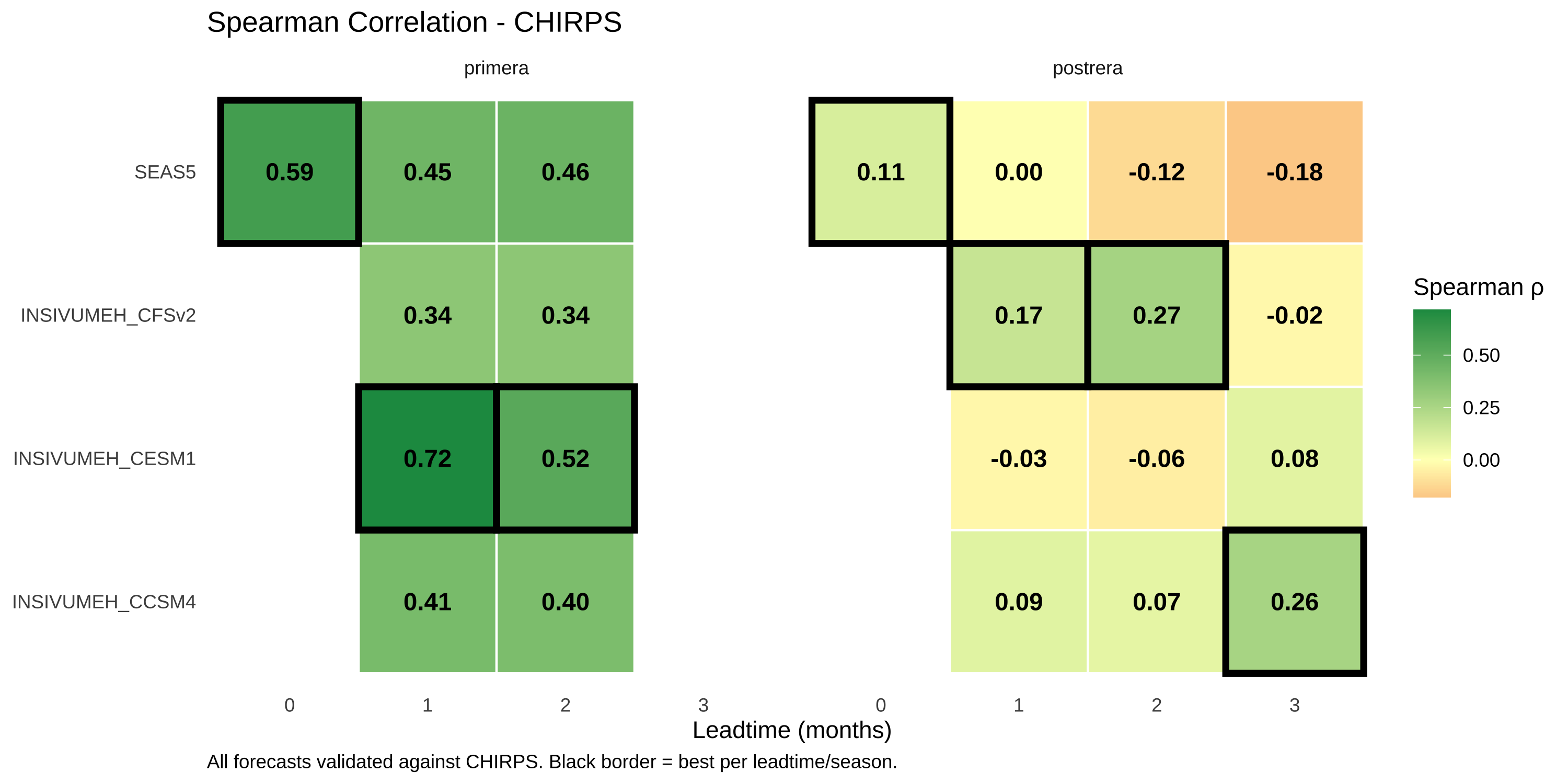
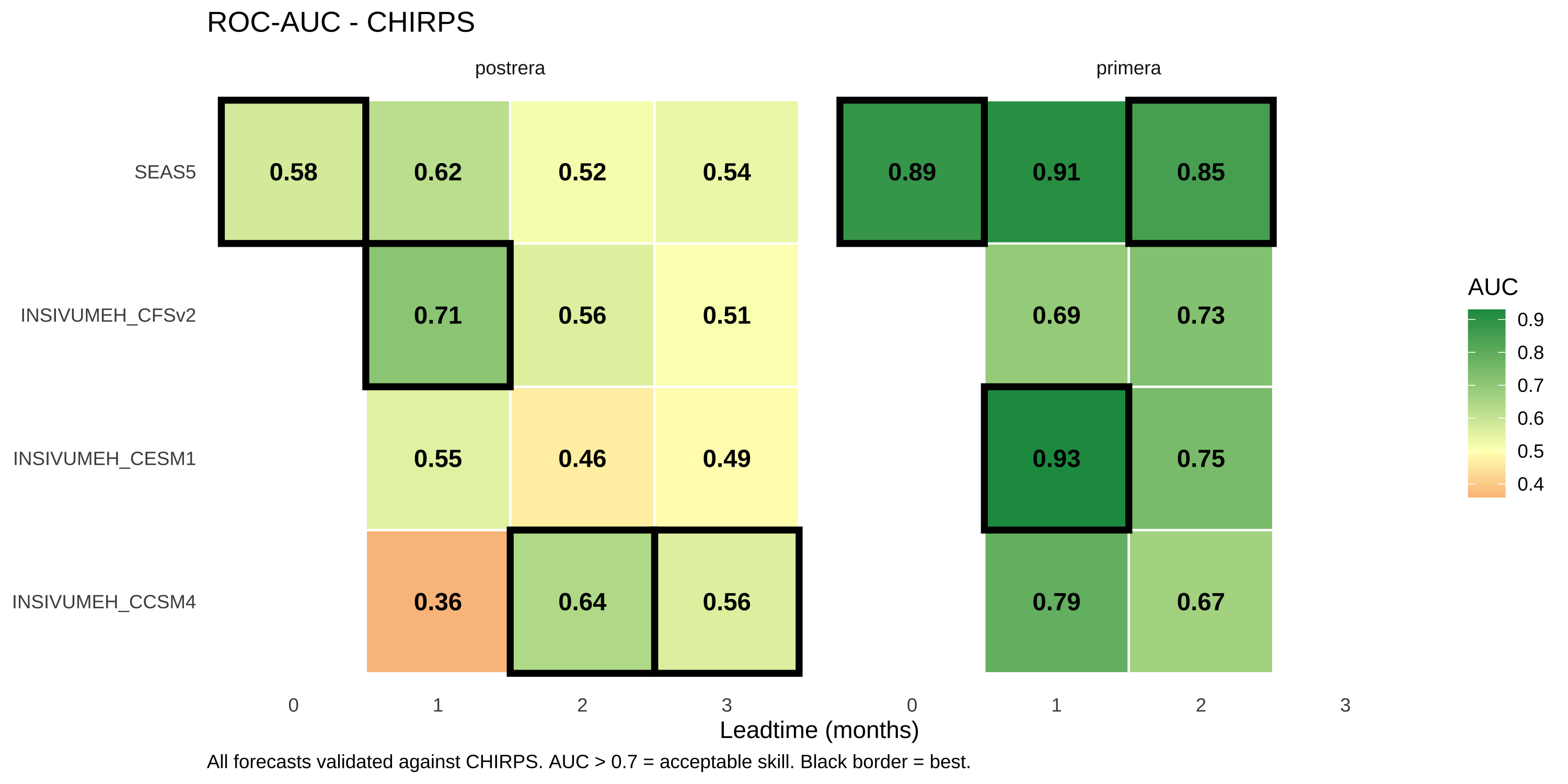
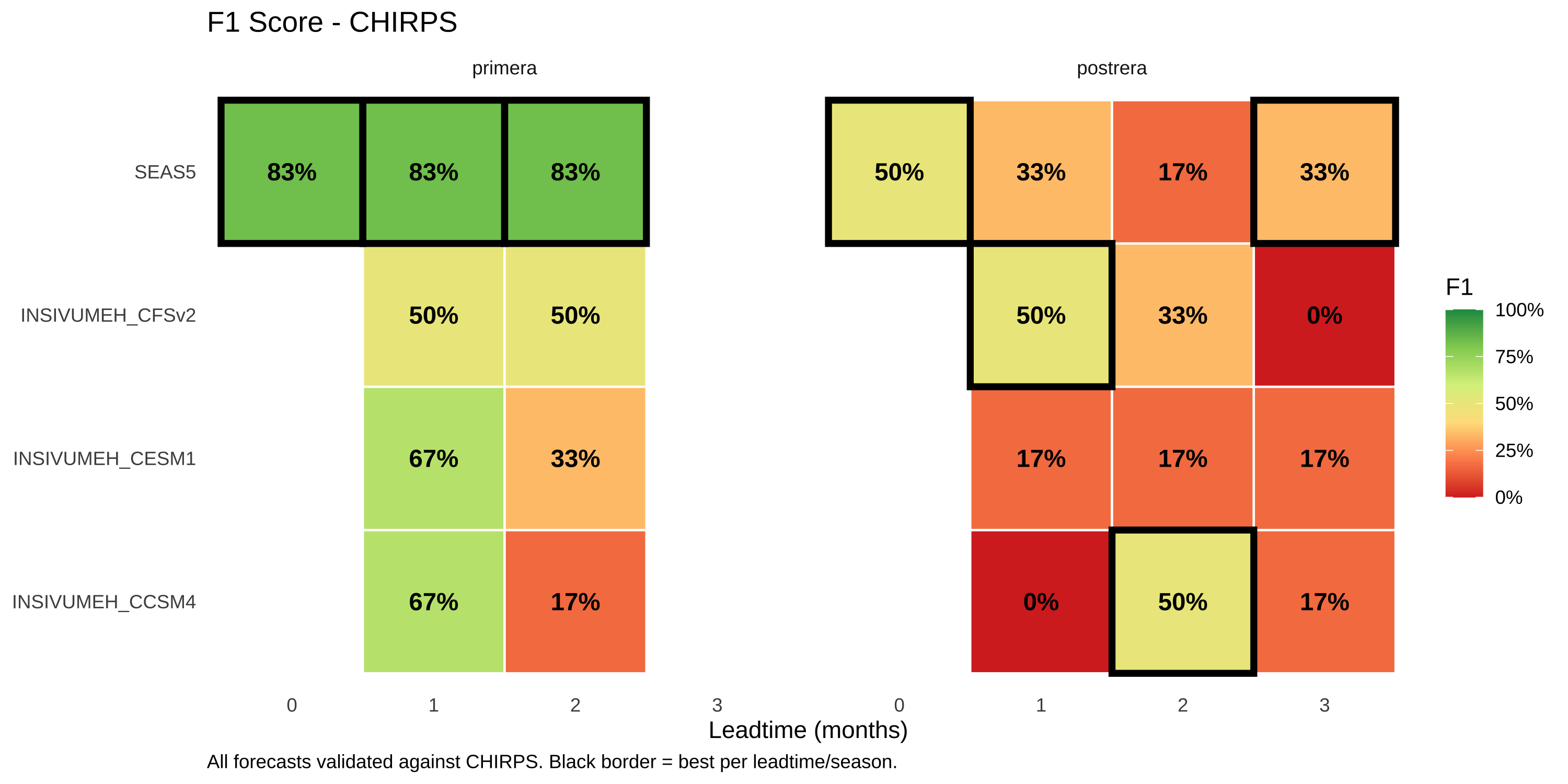
Spearman & ROC-AUC continue to tell a similar story. Models are skillful in primera with SEAS5 as the dominant competitor. Postrera skill remains low, dubious, and messy. Different models win at different leadtimes with some surprising results of INSIVUMEH provided models showing stronger predictive power at greater leadtimes. SEAS5 remains competitive, but less dominant
create_metric_heatmap <-function(df, metric_col, metric_name, title, caption, midpoint =0) { df_plot <- df |>group_by(window, leadtime) |>mutate(is_best =!!sym(metric_col) ==max(!!sym(metric_col), na.rm =TRUE)) |>ungroup() ggplot(df_plot, aes(x =factor(leadtime), y = forecast_source)) +geom_tile(aes(fill =!!sym(metric_col)), color ="white", linewidth =0.5) +geom_tile(data = df_plot |>filter(is_best),fill =NA, color ="black", linewidth =1.5 ) +geom_text(aes(label =sprintf("%.2f", !!sym(metric_col))), size =4, fontface ="bold", color ="black") +facet_wrap(~window) +scale_fill_gradient2(low ="#D73027", mid ="#FFFFBF", high ="#1A9850",midpoint = midpoint, name = metric_name ) +labs(title = title, x ="Leadtime (months)", y =NULL, caption = caption) +theme_minimal() +theme(legend.position ="right", panel.grid =element_blank(),plot.caption =element_text(hjust =0))}create_metric_heatmap(df = df_metrics,metric_col ="spearman",metric_name ="Spearman ρ",title ="Spearman Correlation - CHIRPS",caption ="All forecasts validated against CHIRPS. Black border = best per leadtime/season.")
Surprise finding: INSIVUMEH_CESM1 shows the strongest Spearman correlation for Primera at LT1 (0.72) and LT2 (0.52), outperforming SEAS5. This is the opposite of what we saw with ERA5 and ENACTS.
Primera skill is robust: Multiple models show genuine skill (AUC > 0.7) across all three observation sources. This isn’t an artifact of one particular dataset.
Postrera remains unresolved: No model shows reliable, consistent skill. CCSM4’s apparent better performance at longer leadtimes is suspicious - skill should not improve with leadtime. This inverted pattern is likely noise from the small sample (only ~6 drought events in 25 years).
4.4.2 Open Questions
The tie-breaker analysis raises more questions than it answers for Postrera:
Why the inverted skill pattern? CCSM4 showing better skill at LT2-3 than LT1 is backwards - forecast skill should degrade with leadtime. Is this genuine or noise?
Which model is actually better? With different metrics favoring different models at different leadtimes, we cannot make a confident recommendation.
Is the poor skill a data artifact? Could temporal trends in the observation sources be affecting our skill estimates?
4.4.3 Next Steps
To better understand the poor Postrera skill and the contradictory patterns across models, the next chapter examines temporal drift - whether systematic trends in forecasts or observations might explain some of what we’re seeing.
TipTechnical Details
4.4.4 CHIRPS vs ENACTS Comparison
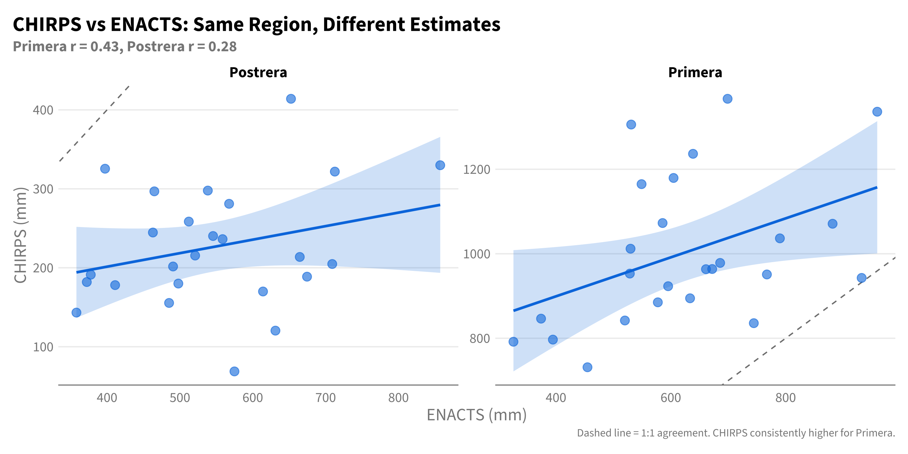
How different are CHIRPS and ENACTS for Chiquimula? Understanding this helps interpret why forecast skill might differ across observation sources.
Compare CHIRPS and ENACTS observations
# Load ENACTS for comparisondf_enacts_compare <- enacts$load_enacts_seasonal("chiquimula")df_compare <- df_chirps |>rename(chirps = obs_mm) |>left_join( df_enacts_compare |>select(year, window, enacts = obs_mm),by =c("year", "window") ) |>filter(!is.na(enacts))# Correlationcorr_primera <- df_compare |>filter(window =="primera") |>summarise(r =cor(chirps, enacts)) |>pull(r)corr_postrera <- df_compare |>filter(window =="postrera") |>summarise(r =cor(chirps, enacts)) |>pull(r)df_compare |>ggplot(aes(x = enacts, y = chirps)) +geom_abline(slope =1, intercept =0, linetype ="dashed", color ="grey50") +geom_point(alpha =0.6, size =3) +geom_smooth(method ="lm", se =TRUE, color ="#007CE1", fill ="#007CE1", alpha =0.2) +facet_wrap(~str_to_title(window), scales ="free") +labs(title ="CHIRPS vs ENACTS: Same Region, Different Estimates",subtitle =sprintf("Primera r = %.2f, Postrera r = %.2f", corr_primera, corr_postrera),x ="ENACTS (mm)",y ="CHIRPS (mm)",caption ="Dashed line = 1:1 agreement. CHIRPS consistently higher for Primera." )
CHIRPS and ENACTS are correlated but not identical. CHIRPS tends to estimate higher rainfall for Primera (~300mm more on average). This means a forecast calibrated to one source may not match the other perfectly - making the three-source comparison a meaningful robustness check.
4.4.5 Forecast Bias
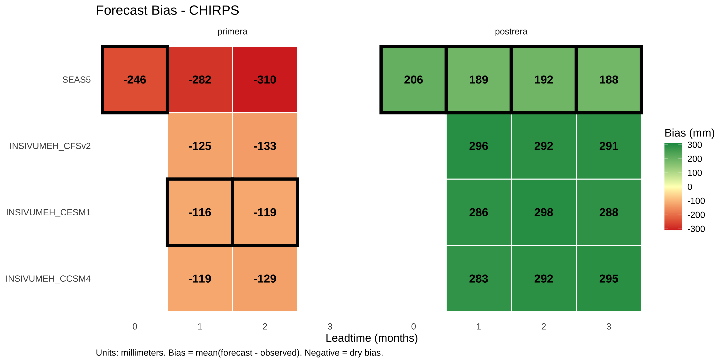
Bias (mean forecast - observed) is shown for completeness, but is not consequential for our framework since we use rank-based metrics and model-specific thresholds rather than raw precipitation values.
Against CHIRPS, all models have dry bias for Primera and wet bias for Postrera. SEAS5 has the largest dry bias for Primera (~280mm under), while INSIVUMEH models are closer (~120mm under).