---
jupyter:
kernelspec:
name: "ds-flood-gfm"
language: "python"
display_name: "ds-flood-gfm"
---
## Global Daily Anomalies
This document demonstrates a proof of concept for querying and visualizing global flood anomalies at scale. We connect to the GFM (Global Flood Monitoring) STAC catalog to identify tiles where flood anomalies have been detected, then visualize the spatial distribution and intensity of these flood events.
The workflow includes:
1. Connecting to the STAC API to query flood anomaly data
2. Filtering for tiles with detected anomalies over recent time periods
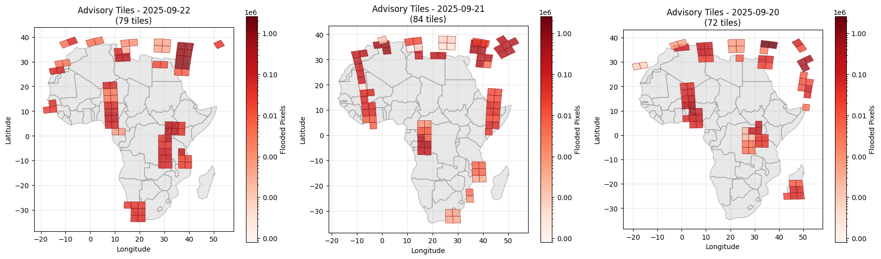
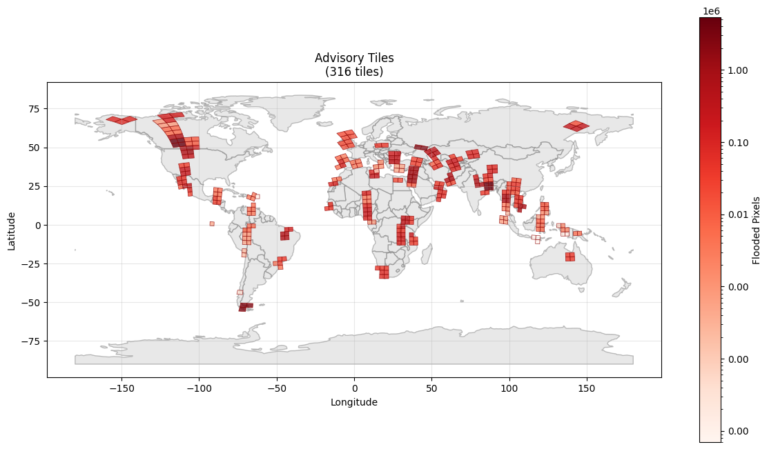
3. Creating visualizations showing flood intensity across Africa and globally
```{python}
import pystac_client
import stackstac
import matplotlib.pyplot as plt
from matplotlib.colors import ListedColormap, BoundaryNorm, LogNorm
import matplotlib.ticker as ticker
import numpy as np
import geopandas as gpd
from ds_flood_gfm.geo_utils import load_adm0_lowres
from shapely.geometry import shape
from datetime import datetime, timedelta
import pandas as pd
from matplotlib.colors import LogNorm

# Configure matplotlib for better display
%matplotlib inline
plt.rcParams['figure.dpi'] = 100
```
## Africa - Last 7 days
We start by analyzing flood anomalies across Africa for the past week. This regional analysis helps us understand the spatial and temporal patterns of flood events across the continent.
```{python}
world = load_adm0_lowres()
gdf_africa = world[world.continent == "Africa"]
gdf_africa_bound = gdf_africa.total_bounds
```
### Connect & Query STAC
We connect to the EODC STAC API and query for GFM tiles covering Africa from September 16-22, 2025. The query specifically filters for tiles where flood anomalies have been detected using the `anomaly_detected` property.
```{python}
stac_api = "https://stac.eodc.eu/api/v1"
client = pystac_client.Client.open(stac_api)

search = client.search(
    collections=["GFM"],
    bbox=gdf_africa_bound,  # Huge geographic extent
    datetime="2025-09-16/2025-09-22",
    query={"anomaly_detected": {"eq": True}},  # Only scenes with advisories
)


item_collection = search.item_collection()
# stack = stackstac.stack(item_collection, epsg=4326)
```
The following code processes the STAC query results to extract flood advisory information. For each tile with detected anomalies, we collect the geometry, timestamp, and flood intensity metrics. We then create daily summaries showing the most severe flooding detected in each tile per day.
```{python}
# Extract advisory geometries and metadata efficiently
advisory_tiles = []
for item in item_collection:
    advisory_tiles.append(
        {
            "geometry": shape(item.geometry),
            "datetime": item.datetime,
            "anomaly_detected": item.properties.get("anomaly_detected", False),
            "flooded_pixels": item.properties.get("flooded_pixels", 0),
            "tile_id": item.properties.get("Equi7Tile"),
            "id": item.id,
        }
    )

# Convert to GeoDataFrame
advisory_gdf = gpd.GeoDataFrame(advisory_tiles)
advisory_gdf["date"] = advisory_gdf["datetime"].dt.date
max_per_day = advisory_gdf.loc[
    advisory_gdf.groupby(["date", "tile_id"])["flooded_pixels"].idxmax()
]


# Optional: Also add a general filter for degenerate geometries
def is_reasonable_geometry(geom):
    bounds = geom.bounds
    width = bounds[2] - bounds[0]
    height = bounds[3] - bounds[1]
    return width < 50 and height < 50 and width > 0.01 and height > 0.01


max_per_day = max_per_day[max_per_day.geometry.apply(is_reasonable_geometry)]
# Filter for the last 3 days and create individual plots


# Get the last 3 days (Sep 21, 20, 19)
target_dates = ["2025-09-22", "2025-09-21", "2025-09-20"]

# Create subplots for the 3 days
fig, axes = plt.subplots(1, 3, figsize=(18, 6))

# Calculate global min/max for consistent color scale
all_data = max_per_day[
    max_per_day["datetime"].dt.date.isin(
        [pd.to_datetime(date).date() for date in target_dates]
    )
]

if len(all_data) > 0:
    # Use log scale for color mapping

    # Get min/max values, ensuring we don't have zeros for log scale
    min_val = max(all_data["flooded_pixels"].min(), 1)  # Avoid log(0)
    max_val = all_data["flooded_pixels"].max()

    # Create log normalizer
    log_norm = LogNorm(vmin=min_val, vmax=max_val)
else:
    log_norm = None
    min_val, max_val = 0, 1

for i, date_str in enumerate(target_dates):
    # Filter data for specific date
    date_data = max_per_day[
        max_per_day["datetime"].dt.date == pd.to_datetime(date_str).date()
    ]

    # Plot on corresponding subplot
    ax = axes[i]

    # Plot Africa first as background
    gdf_africa.plot(ax=ax, color="lightgray", edgecolor="gray", alpha=0.5)

    if len(date_data) > 0:
        # Plot with log-scaled colors but original values in legend
        im = date_data.plot(
            ax=ax,
            column="flooded_pixels",
            cmap="Reds",
            edgecolor="darkred",
            alpha=0.8,
            linewidth=0.5,
            norm=log_norm,
            legend=True,
            legend_kwds={
                "label": "Flooded Pixels",
                "shrink": 0.8,
                "format": ticker.ScalarFormatter(),  # Show actual numbers, not log values
            },
        )
        ax.set_title(f"Advisory Tiles - {date_str}\n({len(date_data)} tiles)")
    else:
        ax.set_title(f"Advisory Tiles - {date_str}\n(No data)")

    ax.set_xlabel("Longitude")
    ax.set_ylabel("Latitude")
    ax.grid(True, alpha=0.3)

plt.tight_layout()
plt.show()
```
## Global - Last Day
Next, we expand our analysis to global scale, focusing on the most recent day (September 22, 2025) to show flood anomalies detected worldwide. This demonstrates the system's capability to monitor flood events at a planetary scale.
```{python}
global_search = client.search(
    collections=["GFM"],
    bbox=np.array([-180, -90, 180, 90]),  # Huge geographic extent
    datetime="2025-09-22/2025-09-22",
    query={"anomaly_detected": {"eq": True}},  # Only scenes with advisories
)


item_collection = global_search.item_collection()
# stack = stackstac.stack(item_collection, epsg=4326)
```
The global visualization uses the same processing approach as the Africa analysis, but shows flood anomalies across all continents. The map uses a logarithmic color scale to effectively display the wide range of flood intensities detected globally.
```{python}
# Extract advisory geometries and metadata efficiently
advisory_tiles = []
for item in item_collection:
    advisory_tiles.append(
        {
            "geometry": shape(item.geometry),
            "datetime": item.datetime,
            "anomaly_detected": item.properties.get("anomaly_detected", False),
            "flooded_pixels": item.properties.get("flooded_pixels", 0),
            "tile_id": item.properties.get("Equi7Tile"),
            "id": item.id,
        }
    )

# Convert to GeoDataFrame
advisory_gdf = gpd.GeoDataFrame(advisory_tiles)
advisory_gdf["date"] = advisory_gdf["datetime"].dt.date
max_per_day = advisory_gdf.loc[
    advisory_gdf.groupby(["date", "tile_id"])["flooded_pixels"].idxmax()
]


# Create single plot for the one date
fig, ax = plt.subplots(1, 1, figsize=(12, 8))

# Calculate min/max for color scale
all_data = max_per_day

if len(all_data) > 0:

    # Get min/max values, ensuring we don't have zeros for log scale
    min_val = max(all_data["flooded_pixels"].min(), 1)  # Avoid log(0)
    max_val = all_data["flooded_pixels"].max()

    # Create log normalizer
    log_norm = LogNorm(vmin=min_val, vmax=max_val)
else:
    log_norm = None
    min_val, max_val = 0, 1

# Plot world as background
world.plot(ax=ax, color="lightgray", edgecolor="gray", alpha=0.5)

if len(max_per_day) > 0:
    # Plot with log-scaled colors but original values in legend
    im = max_per_day.plot(
        ax=ax,
        column="flooded_pixels",
        cmap="Reds",
        edgecolor="darkred",
        alpha=0.8,
        linewidth=0.5,
        norm=log_norm,
        legend=True,
        legend_kwds={
            "label": "Flooded Pixels",
            "shrink": 0.8,
            "format": ticker.ScalarFormatter(),  # Show actual numbers, not log values
        },
    )
    ax.set_title(f"Advisory Tiles\n({len(max_per_day)} tiles)")
else:
    ax.set_title("Advisory Tiles\n(No data)")

ax.set_xlabel("Longitude")
ax.set_ylabel("Latitude")
ax.grid(True, alpha=0.3)

plt.tight_layout()
plt.show()
```