# GFDS vs FloodScan {#sec-alternative-sources}
---
jupyter: ds-flood-gfm
---
The rest of this book is about GFM: 20 m Sentinel-1 flood extent, the right tool
for mapping a flood and estimating exposure. But GFM has structural gaps. Its
revisit pattern leaves 1 to 3 day holes, its archive only starts in 2015, and
continuous global monitoring gets expensive scene by scene. This chapter explores
a complementary source: the Global Flood Detection System (GFDS) behind the
[GDACS flood detection pages](https://www.gdacs.org/flooddetection/download.aspx),
a JRC / Dartmouth Flood Observatory system running since 2006. It is free,
global, daily, and its archive goes back to 1997.
The trade: GFDS is *not* flood extent. It senses passive-microwave brightness
temperature at 36.5 GHz (~10 km pixels) and infers surface-water anomalies,
closer in spirit to FloodScan (which the team licenses) than to GFM. That framing
is exactly why it's interesting: can GFDS serve as a free FloodScan analogue for
admin-level flood monitoring? We test it here against FloodScan SFED over the
Nigeria 2022 floods. The full source evaluation lives in
[`docs/gdacs-gfds-assessment.md`](https://github.com/OCHA-DAP/ds-flood-gfm/blob/main/docs/gdacs-gfds-assessment.md).
## How GFDS works, in one section
Water emits far less microwave radiation than dry land, so a flooding pixel looks
"colder" at 36.5 GHz. Raw brightness temperature also wobbles with weather, so
GFDS always ratios a river measurement pixel **M** against a nearby dry
calibration pixel **C** experiencing the same atmosphere:
$$s = T_M / T_C$$
Lower signal means more water. The server exposes half a dozen layers; after
taking them apart, only one needs continuous ingestion, plus two static files:
| Layer | What it is | Used in this chapter? |
|---|---|---|
| `SignalTiffs/signal_*` | daily $s$ (×10⁶, int32) | **Yes**: the input to every analysis and plot below |
| `AveragesAndSd/bt_signal_{avg,sd}` | per-pixel long-term mean/sd of $s$, static since July 2009 | **Yes**: fetched once, used to score the signal into an anomaly |
| `MagTiffs/mag_signal_*` | $s$ scored in σ against JRC's baseline | Only in the final head-to-head section, as the thing we test against |
| `Avg*` folders | 4-day trailing means of the above | Never downloaded; we compute our own 4-day mean in one line of xarray |
| `dn_*`, `deltaT_*` | legacy formulations | No |
Two data-hygiene facts you need before touching any of it: rasters carry two
nodata sentinels (`-32000` declared, int32-min undeclared), and every layer is
int32 with a scale factor (signal ×1,000,000; magnitude ×1,000).
JRC's own documentation is two reports: the
[2015 data-product specification](https://www.gdacs.org/flooddetection/Download/Technical_Note_GFDS_Data_Products_v1.pdf)
(De Groeve, Brakenridge, Paris) and the 2007 system description with
validation ([Kugler & De Groeve, EUR 23303](https://www.unisdr.org/files/9622_LBNA23303ENC002.pdf)).
The 2007 validation against 58 major flood events is sobering and useful:
35 to 42% of monitored sites gave a clean, reliable signal, roughly another
third detected the flood through heavy noise, 14 to 16% missed it, and Sahel
irrigation was already flagged as a false-alarm source. The 4 to 6σ
"extreme flood" thresholds were set empirically and marked as needing
confirmation. The operational GFDS mitigates all this with manually curated
sites; the gridded rasters we use below share the same physics but none of
that site-level curation, which is why we validate before trusting them.
A status note obtained directly from the JRC team (September 2026): the
project was completed around 2015 and has run without further updates since;
the visualization interface has been decommissioned, while the data services
we use remain online, and a transfer of the system to the Dartmouth Flood
Observatory group at the University of Colorado has been under discussion
for years. In plain terms, the feed works but nobody maintains it. That
explains the frozen 2009 baseline and argues for archiving the data while
the service lasts; the deeper mitigation is that GFDS is a processing chain
over public AMSR2/GPM brightness temperatures, so the signal could be
recomputed from source if the feed stops.
## Sensors and methods, side by side
Before comparing outputs, it is worth being precise about what each system
actually measures and how. The two are cousins, not strangers: they observe
the same physical signal from largely the same instruments, then diverge
completely in what they do with it.
| | **GFDS** (JRC / DFO) | **FloodScan** (AER) |
|---|---|---|
| Sensors today | AMSR2 (GCOM-W), GMI (GPM) | AMSR2 (GCOM-W), GMI (GPM) |
| Historical sensors | AMSR-E (2002 to 2011), TRMM TMI (1997 to 2015) | AMSR-E era products |
| Observable | 36.5 GHz H-pol brightness temperature, per swath | Passive microwave brightness temperature, same 36 GHz-class channels |
| Native footprint at 36 GHz | AMSR2: 7×12 km; GMI: 9.4×15.6 km ([JAXA](https://www.eorc.jaxa.jp/AMSR/resources/pdf/amsr2_data_user_guide_v4.pdf), [NASA](https://gpm.nasa.gov/missions/GPM/GMI)) | Identical (shared instruments) |
| Working resolution before any downscaling | Posted to the 0.09° (~10 km) grid, close to native | Intermediate flooded fraction produced "at the passive microwave satellite data scales (~22-km)" (FloodScan Data Users Guide v05R01, AER 2021, §1.2) |
| Core retrieval | Change detection: wet pixel ÷ nearby dry calibration pixel (M/C ratio), a unitless relative signal | Unmixing: wet/dry emissivity end-members convert Tb into a physical *fraction of pixel flooded* |
| Reference for "dry" | One calibration pixel, chosen as the 95th percentile of a 9×9 neighborhood, same swath | Dry-land end-member predicted per location from local time-series analysis |
| Long-term baseline | Static per-pixel mean/sd, frozen July 2009 (AMSR-E era) | Maintained dynamically as part of the retrieval |
| Spatial treatment | Swath values projected to the grid as-is; no downscaling | Physical downscaling to 90 m via a topography / hydrology / Global Surface Water database, then aggregation |
| Grid we use | 0.09° (~10 km), 4000×2000 global | 300 arcsec (~0.083°, ~9 km); 90 m product also exists |
| Noise handling | 4-day trailing average (chosen over spatial averaging in the 2007 report) | Temporal-spatial false-positive filtering plus 3-day averaging |
| Coverage | Global (40°N to 40°S in the TRMM-only era, 1997 to 2002) | Africa and the Americas in NRT, not global |
| Cadence / latency | Daily grids, updated every 3 h; ~3 h (AMSR2) to ~24 h (GPM) behind acquisition | Daily |
| Archive | December 1997 to present | 1998 to present (team holdings) |
| Output variable | σ-anomaly of a wetness ratio; no physical units | Flooded fraction, 0 to 1 (SFED; MFED for maximum) |
| Alert layer | ~10k manually curated virtual-gauge sites; 4 to 6σ thresholds set empirically | Products consumed directly; the team computes its own baselines and return periods |
| Access | Free, no auth, plain HTTP | Commercial license (AER) |
A detail in that table deserves emphasis, because it inverts the intuition
the two products' grids give you. The raw radiometry is identical, roughly 7
to 16 km footprints from the same two instruments. From there the systems
move in opposite directions: GFDS keeps close to native resolution (~10 km
posting) and never downscales, while FloodScan first *coarsens* to ~22 km
effective for a stable retrieval and only then paints 90 m detail from its
hydrological database. FloodScan's fine appearance is entirely prior
knowledge about where water goes, not finer measurement; at the radiometric
level GFDS actually retains slightly more spatial information.
Three things follow from this table.
First, the r ≈ 0.9 agreements we find below are impressive but not fully
independent evidence: both systems see the world through the same
radiometers. Shared blind spots (coasts, snow, heavy vegetation, swath gaps)
will not show up as disagreement between them. FloodScan is our
operational benchmark here, not ground truth; truly independent validation
would come from SAR extent (GFM) or gauges.
Second, the methodological gulf explains the asymmetries we measure. A ratio
anomaly is only meaningful relative to a pixel's own history, so GFDS values
cannot be compared across pixels as amounts of water, and anything that
shifts local emissivity (irrigation, seasonal wetlands, coastlines) moves the
signal. A flooded *fraction* is a physical quantity: comparable across
pixels, aggregatable into areas and exposure, and, thanks to the 90 m
hydrological downscaling, able to keep narrow river corridors that are
sub-pixel at the radiometer's native footprint.
Third, GFM belongs to a different family altogether: an active C-band SAR
(Sentinel-1) classifying 20 m flood extent per scene, with revisit gaps and a
2015-start archive. That is why this chapter compares GFDS against FloodScan
rather than GFM; the systems in this table answer "how unusual is the water
signal today, everywhere, daily", while GFM answers "exactly where is the
water right now".
## Data access: long fetches live in scripts
Downloading a season is slow and flaky. During this work the GDACS server swung
from ~2 s to ~140 s per file within a single day. So the fetch steps live in
standalone, resumable scripts (throttled, per-day `.npy` cache, a 404 recorded as
a `.missing` marker, any other error raising loudly). The chapter then runs
reproducibly off the local cache. The scripts are shown here but not executed
at render time:
```{python}
#| eval: false
#| code-summary: "experiments/gfds_nga2022/fetch_gfds_nga.py — GFDS signal + magnitude + baselines"
{{< include ../experiments/gfds_nga2022/fetch_gfds_nga.py >}}
```
```{python}
#| eval: false
#| code-summary: "experiments/gfds_nga2022/fetch_sfed_nga.py — FloodScan SFED from team blob"
{{< include ../experiments/gfds_nga2022/fetch_sfed_nga.py >}}
```
## The test case: Nigeria, June to December 2022
A near-ideal reference event: [Lagdo Dam releases from 13 September
2022](https://reliefweb.int/report/nigeria/acaps-briefing-note-nigeria-country-wide-flooding-21-october-2022),
the Niger-Benue confluence (Lokoja) peaking early to mid October, Bayelsa
flooding downstream into November. We know where and when, so we can score GFDS
against FloodScan at the places that mattered.
```{python}
#| code-summary: "load cached stacks (fails loudly if the fetch scripts haven't been run)"
from pathlib import Path

import matplotlib.pyplot as plt
import numpy as np
import pandas as pd
import xarray as xr

CACHE = next(
    (p for p in (Path("data/gdacs_gfds/nga2022"),
                 Path("../data/gdacs_gfds/nga2022")) if p.exists()),
    None,
)
if CACHE is None:
    raise FileNotFoundError(
        "GFDS cache not found. Run experiments/gfds_nga2022/fetch_gfds_nga.py "
        "and fetch_sfed_nga.py from the repo root first (they are resumable)."
    )
SENTINELS = (-32000, -2147483648)


def gfds_coords(shape):
    a, b, c, d, e, f = np.load(CACHE / "geotransform.npy")
    xs = c + (np.arange(shape[1]) + 0.5) * a
    ys = f + (np.arange(shape[0]) + 0.5) * e
    return xs, ys


def load_stack(prefix, scale, positive_only):
    files = sorted(CACHE.glob(f"{prefix}_2022*.npy"))
    arrs, dates = [], []
    for p in files:
        dates.append(pd.Timestamp(p.stem.split("_")[-1]))
        a = np.load(p).astype("float64")
        bad = np.isin(a, SENTINELS)
        if positive_only:
            bad |= a <= 0
        a[bad] = np.nan
        arrs.append(a / scale)
    xs, ys = gfds_coords(arrs[0].shape)
    return xr.DataArray(np.stack(arrs), dims=("time", "y", "x"),
                        coords={"time": dates, "y": ys, "x": xs})


signal = load_stack("signal", 1_000_000, positive_only=True)
mag = load_stack("mag", 1_000, positive_only=False)

co = np.load(CACHE / "sfed_coords.npz")
sfed_files = sorted(CACHE.glob("sfed_2022*.npy"))
sfed = xr.DataArray(
    np.stack([np.load(p) for p in sfed_files]),
    dims=("time", "y", "x"),
    coords={"time": [pd.Timestamp(p.stem.split("_")[-1]) for p in sfed_files],
            "y": co["y"], "x": co["x"]},
)

baseline = {}
for which in ("avg", "sd"):
    b = np.load(CACHE / f"baseline_{which}.npy").astype("float64")
    b[np.isin(b, SENTINELS) | (b <= 0)] = np.nan
    xs, ys = gfds_coords(b.shape)
    baseline[which] = xr.DataArray(b / 1_000_000, dims=("y", "x"),
                                   coords={"y": ys, "x": xs})

print(f"signal: {signal.sizes['time']} days | mag: {mag.sizes['time']} days "
      f"| sfed: {sfed.sizes['time']} days | grid {signal.sizes['y']}x{signal.sizes['x']}")
```
### A do-it-yourself anomaly
To be explicit about lineage, since the server offers half a dozen layers:
everything from here on is built from exactly three GFDS inputs. The daily
`signal_*` files provide $s$; the two static baseline files provide the
per-pixel mean and sd. We score the signal flood-positive (floods lower it),
and then compute the 4-day trailing mean ourselves, on the anomaly, in the
`rolling` call below. JRC's pre-computed `Avg*` layers play no part, and its
`mag_signal_*` product appears only at the end, as a comparison target.
Single GFDS days are swath-based and noisy, which is why the smoothed version
earns its keep.
```{python}
anom = ((baseline["avg"] - signal) / baseline["sd"].clip(min=0.005)).transpose(
    "time", "y", "x"
)
anom4 = anom.rolling(time=4, min_periods=1).mean()
sfed_g = sfed.interp(x=signal.x, y=signal.y, method="linear")  # onto GFDS grid
```
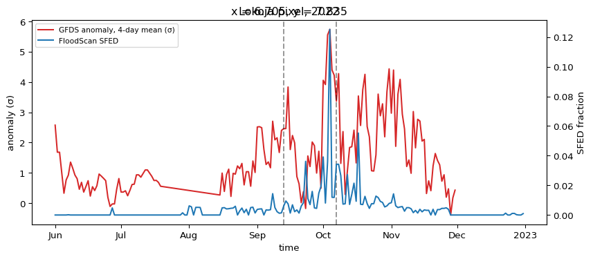
### Sanity check: the Lokoja pixel
```{python}
#| fig-cap: "GFDS anomaly vs FloodScan SFED at the Niger-Benue confluence. Dashed lines: Lagdo Dam release (13 Sep) and the documented Kogi peak week."
fig, ax = plt.subplots(figsize=(10, 4))
pt = dict(x=6.74, y=7.80, method="nearest")
anom4.sel(**pt).plot(ax=ax, color="tab:red", label="GFDS anomaly, 4-day mean (σ)")
ax2 = ax.twinx()
sfed_g.sel(**pt).plot(ax=ax2, color="tab:blue", label="FloodScan SFED")
ax2.set_ylabel("SFED fraction")
ax.set_ylabel("anomaly (σ)")
for dt in ("2022-09-13", "2022-10-07"):
    ax.axvline(pd.Timestamp(dt), ls="--", color="k", alpha=0.4)
ax.set_title("Lokoja pixel, 2022")
h1, l1 = ax.get_legend_handles_labels()
h2, l2 = ax2.get_legend_handles_labels()
ax.legend(h1 + h2, l1 + l2, loc="upper left", fontsize=8)
plt.show()
```
The anomaly climbs from mid-August, surges after the dam release, and peaks in
the documented peak week. Not bad for a 10 km radiometer ratio scored against a
17-year-old baseline. Encouraging enough to score it properly.
### Where does GFDS agree with FloodScan?
A note on method before the maps: the correlation below is a plain Pearson r
on the continuous daily values. Per pixel, we correlate the 4-day-mean GFDS
anomaly (σ) against SFED (fraction) over the days where both are finite,
requiring at least 60 shared days. SFED is first resampled (bilinear) from
its native 0.083° grid onto the GFDS 0.09° grid, so every pixel-level
comparison in this chapter happens on the GFDS grid. Nothing is classified
or thresholded before
correlating; thresholds appear only afterwards, to stratify the results by
how much flooding a pixel actually saw.
```{python}
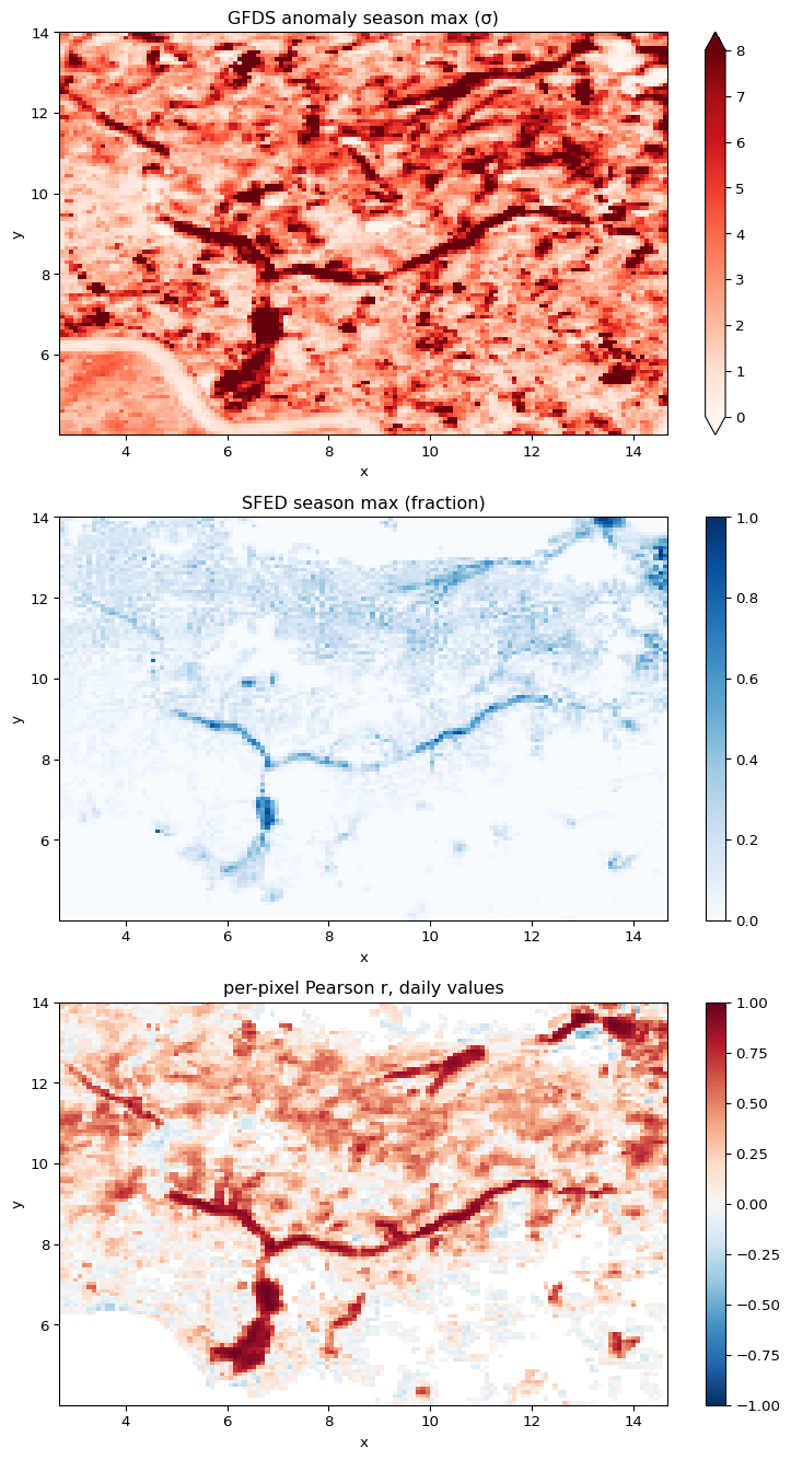
#| fig-cap: "Top: GFDS anomaly seasonal max. Middle: FloodScan SFED seasonal max (resampled to the GFDS 0.09° grid, as in all pixel comparisons here). Bottom: per-pixel Pearson correlation of the daily series. GFDS lights up far more area than SFED; the correlation map shows where that extra signal tracks real flooding (river corridors) and where it does not."
#| fig-height: 14
def pixel_corr(a_stack, b_stack, min_days=60):
    a2, b2 = xr.align(a_stack, b_stack)
    A = a2.values.reshape(a2.sizes["time"], -1)
    B = b2.values.reshape(b2.sizes["time"], -1)
    both = np.isfinite(A) & np.isfinite(B)
    out = np.full(A.shape[1], np.nan)
    for j in np.where(both.sum(0) >= min_days)[0]:
        m = both[:, j]
        if A[m, j].std() > 1e-6 and B[m, j].std() > 1e-6:
            out[j] = np.corrcoef(A[m, j], B[m, j])[0, 1]
    return xr.DataArray(out.reshape(a2.shape[1:]), dims=("y", "x"),
                        coords={"y": a2.y, "x": a2.x}), a2, b2


corr, anom_i, sfed_i = pixel_corr(anom4, sfed_g)
gfds_max, sfed_max = anom_i.max("time"), sfed_i.max("time")

fig, axes = plt.subplots(3, 1, figsize=(8, 14))
gfds_max.plot(ax=axes[0], vmin=0, vmax=8, cmap="Reds")
axes[0].set_title("GFDS anomaly season max (σ)")
sfed_max.plot(ax=axes[1], vmin=0, vmax=1, cmap="Blues")
axes[1].set_title("SFED season max (fraction)")
corr.plot(ax=axes[2], vmin=-1, vmax=1, cmap="RdBu_r")
axes[2].set_title("per-pixel Pearson r, daily values")
plt.tight_layout()
plt.show()

flooded = (sfed_max > 0.2).values.ravel()
cv = corr.values.ravel()
print(f"median r, all pixels: {np.nanmedian(cv):.2f} | "
      f"flooded pixels (SFED max>0.2): {np.nanmedian(cv[flooded]):.2f}")
```
Reading the three panels together, not just the corridors:
- GFDS is a sensitive but unspecific wet-season detector. The top panel
shows the Niger-Benue system clearly, but also broad signal above 3σ across
much of the country, strongest in the northern band where seasonal wetlands
(e.g. the Hadejia-Yobe system) saturate every rainy season. SFED (middle)
is far more surgical: river corridors and little else. GFDS's 36.5 GHz
ratio responds to any increase in surface water or saturation, not just
inundation of the kind FloodScan is calibrated for.
- The correlation map is what separates the two kinds of GFDS signal.
Along the major corridors it is dark red (r ≈ 0.9); across the northern
wetland band it is moderate (0.4 to 0.7, both products breathing with the
season); and in the interfluve south-centre it fades to noise.
- The pale stripe hugging the coastline in the top panel is the ocean
contamination effect: sea water in the 10 km footprint wrecks the wet/dry
calibration contrast. This is Ekeremor's failure (next section) visible as
geography.
The disagreements are worth quantifying, because they define what GFDS must
not be used for:
```{python}
#| code-summary: "cross-tab: where each product flags high"
gf_hi = (gfds_max > 3).values.ravel()
sf_hi = flooded
ok = np.isfinite(gfds_max.values.ravel()) & np.isfinite(sfed_max.values.ravel())
tab = pd.DataFrame(
    [[int((gf_hi & sf_hi & ok).sum()), int((gf_hi & ~sf_hi & ok).sum())],
     [int((~gf_hi & sf_hi & ok).sum()), int((~gf_hi & ~sf_hi & ok).sum())]],
    index=["GFDS > 3σ", "GFDS ≤ 3σ"],
    columns=["SFED > 0.2", "SFED ≤ 0.2"],
)
print(tab)
print(f"\nmedian r — both high: {np.nanmedian(cv[gf_hi & sf_hi & ok]):.2f} | "
      f"GFDS-only: {np.nanmedian(cv[gf_hi & ~sf_hi & ok]):.2f} | "
      f"SFED-only: {np.nanmedian(cv[~gf_hi & sf_hi & ok]):.2f}")
```
Two asymmetric failure modes:
- GFDS-only pixels outnumber joint detections about 3.5 to 1, and within them
the daily correlation with SFED collapses to roughly 0.2. A naive "alert
where anomaly exceeds 3σ" rule would therefore over-flag dramatically. This
matches what we measured globally on the live product (on an ordinary day,
~2% of valid land pixels exceed the 4σ "RED" level, over half of them
high-latitude snow and ice; see the assessment doc), and it matches JRC's
own 2007 validation, where the 4 to 6σ extreme-flood thresholds were set
empirically and flagged for confirmation, with Sahel irrigation noted as a
known false-alarm source. The anomaly is meaningful as a time series in
known riverine areas, not as a standalone exceedance map.
- The SFED-only pixels cluster in the far north (median ~12°N): the
narrow Sokoto-Rima and Hadejia channels, where a flooding river is simply
sub-pixel for a 10 km microwave footprint. GFDS reports the coarse ratio
as-is, with no spatial prior to recover small features. FloodScan does:
its published product is downscaled to 90 m using a database built from
topography, hydrology, and Global Surface Water occurrence
([Galantowicz 2018](https://ui.adsabs.harvard.edu/abs/2018AGUFM.H51B..03G/abstract)),
then aggregated to the 300-arcsecond grid we use, so narrow channels
survive in SFED.
### The test that matters: admin level
The team's operational pattern (e.g. `floodscan_exposure`) is a daily zonal
statistic per admin unit. We aggregate both products to Nigeria's 774 LGAs over
the complete event window and score each LGA on correlation and timing.
Timing needs care. The obvious metric, day of GFDS maximum minus day of SFED
maximum, turned out to be fragile: a single noisy spike moves the argmax, and
the 4-day trailing mean shifts GFDS peaks late by construction. For the same
LGA it flipped by up to 16 days depending only on the smoothing choice. We
use the lag that maximises the cross-correlation between the two daily series
(bounded at ±15 days) instead, which was stable across smoothing choices in
our checks. Positive lag means GFDS moves later than SFED.
```{python}
#| code-summary: "daily zonal means per LGA (few minutes; frozen after first render)"
import ocha_stratus as stratus
from rasterio.transform import from_bounds as tf_from_bounds
from rasterstats import zonal_stats

adm2 = stratus.codab.load_codab_from_blob("nga", admin_level=2)

a4 = anom4.sel(time=slice("2022-08-15", "2022-11-30"))
sf = sfed_g.sel(time=slice("2022-08-15", "2022-11-30"))
if a4.y.values[0] < a4.y.values[-1]:
    a4, sf = a4.isel(y=slice(None, None, -1)), sf.isel(y=slice(None, None, -1))
res_deg = 0.09
affine = tf_from_bounds(
    float(a4.x.min()) - res_deg / 2, float(a4.y.min()) - res_deg / 2,
    float(a4.x.max()) + res_deg / 2, float(a4.y.max()) + res_deg / 2,
    a4.sizes["x"], a4.sizes["y"],
)

rows = []
for ts in pd.to_datetime(a4.time.values):
    za = zonal_stats(adm2, a4.sel(time=ts).values, affine=affine,
                     nodata=np.nan, all_touched=True, stats="mean")
    zs = zonal_stats(adm2, sf.sel(time=ts).values, affine=affine,
                     nodata=np.nan, all_touched=True, stats="mean")
    for pc, lga, st, g, s in zip(adm2.ADM2_PCODE, adm2.ADM2_EN, adm2.ADM1_EN,
                                 (z["mean"] for z in za), (z["mean"] for z in zs)):
        rows.append({"date": ts, "pcode": pc, "lga": lga, "state": st,
                     "gfds": g, "sfed": s})
lga_daily = pd.DataFrame(rows)
```
```{python}
#| code-summary: "score each LGA: correlation + cross-correlation lag"
def best_lag(a, b, max_lag=15):
    """Lag (days) maximising corr(a shifted by L, b). Positive = a later."""
    best, best_r = np.nan, -np.inf
    for L in range(-max_lag, max_lag + 1):
        r = a.shift(L).corr(b)
        if pd.notna(r) and r > best_r:
            best_r, best = r, L
    return best


per = []
for (pc, lga, st), sub in lga_daily.groupby(["pcode", "lga", "state"]):
    sub = sub.dropna(subset=["gfds", "sfed"]).sort_values("date")
    if len(sub) < 60:
        continue
    per.append({
        "lga": lga, "state": st,
        "r": sub["gfds"].corr(sub["sfed"]),
        "xcorr_lag_days": best_lag(sub["gfds"].reset_index(drop=True),
                                   sub["sfed"].reset_index(drop=True)),
        "sfed_max": sub["sfed"].max(),
    })
scores = pd.DataFrame(per)

bands = [(0.02, 0.05), (0.05, 0.10), (0.10, 0.20), (0.20, 1.0)]
summary = pd.DataFrame([
    {"SFED max band": f"{lo:.2f}–{hi:.2f}",
     "median r": round(b.r.median(), 2),
     "median |xcorr lag| (d)": b.xcorr_lag_days.abs().median(),
     "n LGAs": len(b)}
    for lo, hi in bands
    if len(b := scores[(scores.sfed_max > lo) & (scores.sfed_max <= hi)])
])
summary
```
Correlation rises monotonically with flood severity, and the timing alignment
tightens with it. That is the signature of a real shared signal rather than a
lucky fit. One honest framing caveat: 2022 in this basin is essentially a
single flood wave, so these correlations measure agreement on one event's
rise, peak, and recession, computed over the full daily series, not skill
across many independent events. (The season-max maps above are used only for
display and stratification.) A multi-year replication is the obvious next
step. And in the LGAs we know flooded:
```{python}
REF = ["Lokoja", "Ajaokuta", "Ibaji", "Bassa", "Kogi",
       "Yenegoa", "Sagbama", "Ekeremor"]  # CODAB spells Yenagoa 'Yenegoa'
(scores[scores.lga.isin(REF)]
 .sort_values("r", ascending=False)
 .round({"r": 2, "sfed_max": 3})
 .reset_index(drop=True))
```
```{python}
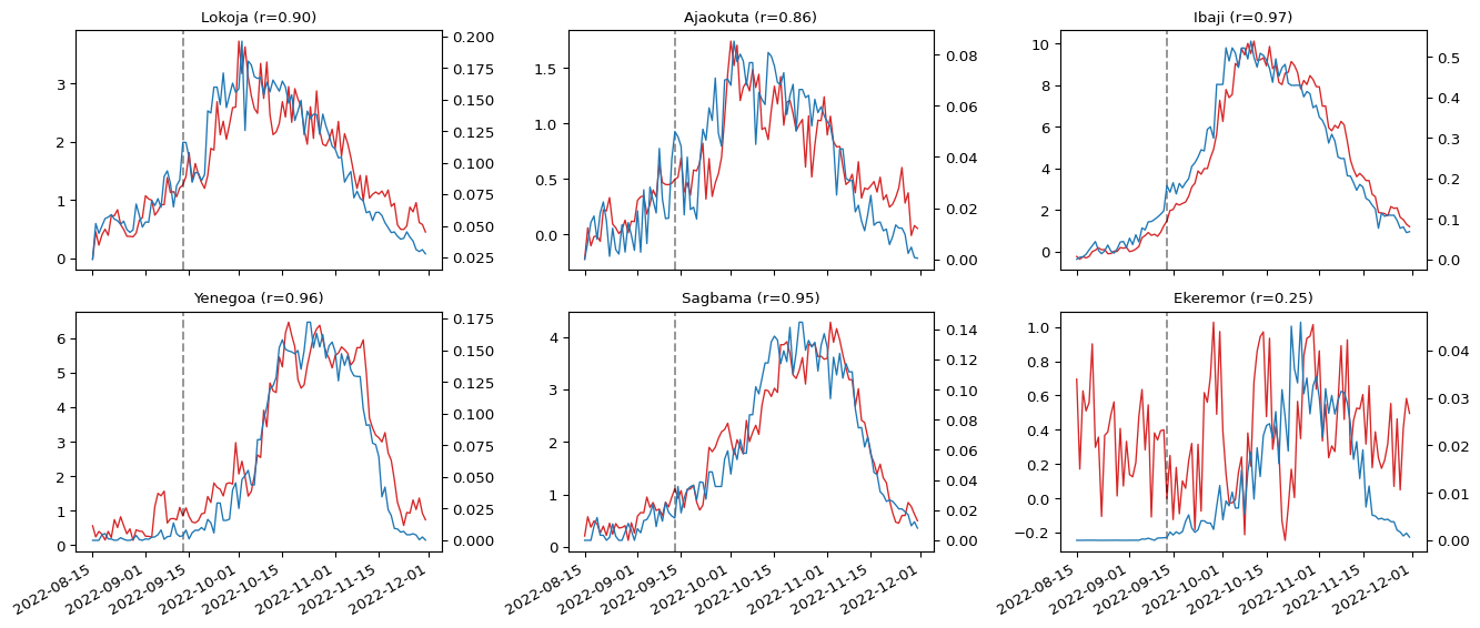
#| fig-cap: "Reference LGAs: GFDS anomaly (red, left axis) vs FloodScan SFED (blue, right axis). Dashed line: Lagdo Dam release."
fig, axes = plt.subplots(2, 3, figsize=(14, 6), sharex=True)
for ax, lga in zip(axes.ravel(),
                   ["Lokoja", "Ajaokuta", "Ibaji", "Yenegoa", "Sagbama", "Ekeremor"]):
    sub = lga_daily[lga_daily.lga == lga].sort_values("date")
    ax.plot(sub.date, sub.gfds, color="tab:red", lw=1)
    ax2 = ax.twinx()
    ax2.plot(sub.date, sub.sfed, color="tab:blue", lw=1)
    row = scores[scores.lga == lga]
    ax.set_title(f"{lga} (r={row.r.iloc[0]:.2f})" if len(row) else lga, fontsize=10)
    ax.axvline(pd.Timestamp("2022-09-13"), ls="--", c="k", alpha=0.4)
fig.autofmt_xdate()
plt.tight_layout()
plt.show()
```
The confluence LGAs track FloodScan curve for curve (r = 0.89 to 0.97, with
cross-correlation lags within 3 days). The instructive failure is Ekeremor: a
coastal delta LGA where the 10 km microwave footprint mixes with ocean and
estuary, so GFDS never gets the dry land calibration contrast its physics
requires. Coastal admin units sit outside its trust region. FloodScan's own
Users Guide draws the same boundary for itself: "flooding in smaller
floodplains and within 5-10 km of coastlines is usually not depicted"
(v05R01, §1.1). This is a limitation of the shared physics, not of either
implementation.
### Do we need JRC's magnitude layer at all?
JRC publishes its own σ-scored product (`mag_signal`), computed against a
baseline frozen in July 2009 and built from a sensor (AMSR-E) that died in
2011. If our DIY anomaly matches it, ingestion only needs the raw signal.
```{python}
corr_mag, _, _ = pixel_corr(mag, sfed_g)
cm = corr_mag.values.ravel()
print(f"median r vs SFED over flooded pixels — "
      f"DIY anomaly: {np.nanmedian(cv[flooded]):.2f} | "
      f"JRC magnitude: {np.nanmedian(cm[flooded]):.2f}")
```
On this event the DIY anomaly clearly beats JRC's own magnitude, which is what
you'd expect when modern AMSR2/GPM measurements are scored against an
AMSR-E-era baseline. The staleness that makes GFDS's global alerting noisy
(documented in the assessment) costs it here too. Ingest the raw signal only
and score it ourselves.
## What this settles
1. Ingest one layer: daily `signal`, roughly 13 MB/day re-encoded as a uint16
COG, plus the two static baseline files fetched once. Magnitude, the 4-day
averages, and the legacy layers are all derivable or ignorable.
2. The common data model fits directly. A daily zonal mean of the 4-day
smoothed anomaly per admin unit has the same `(pcode, date, value)` shape
as the team's `floodscan_exposure` table.
3. The trust region is measured, not guessed: substantial riverine flooding.
Among LGAs whose SFED max passed 0.10, 58% correlate at r ≥ 0.6; past
0.20 the median r is 0.75. Coastal units, marginal flooding, and
single-day values sit outside it.
4. The static 2009 baseline is enough for within-season tracking. Cross-season
return periods want a day-of-year climatology computed from the 2015+
AMSR2/GPM archive, which the assessment verified is complete.
Bottom line: raw GFDS signal, scored and aggregated ourselves, is a credible
free FloodScan analogue for admin-level riverine flood monitoring, with an
archive from 1997 to present at roughly 3 hour latency. The one operational
caveat is the 2009-era GDACS server, which demands resumable, patient
ingestion.