---
jupyter: ds-flood-gfm
---
## Simple STAC based approach to recent composites
```{python}
import pystac_client
import stackstac
import matplotlib.pyplot as plt
from matplotlib.colors import ListedColormap, BoundaryNorm
import numpy as np
import geopandas as gpd
from fsspec.implementations.http import HTTPFileSystem
from ds_flood_gfm.geo_utils import load_adm0_lowres
import time

# Configure matplotlib for better display
%matplotlib inline
plt.rcParams['figure.dpi'] = 100
```
## Area of Interest
Define spatial and temporal range for flood analysis. We'll use Adamawa State, Nigeria for September 2025.
```{python}
GLOBAL_ADM1 = (
    "https://data.fieldmaps.io/edge-matched/humanitarian/intl/adm1_polygons.parquet"
)
ISO3 = "NGA"
filesystem = HTTPFileSystem()
filters = [("iso_3", "=", ISO3)]
gdf = gpd.read_parquet(GLOBAL_ADM1, filesystem=filesystem, filters=filters)
gdf_aoi = gdf[gdf.adm1_name == "Adamawa"]
```
```{python}
gdf_world_adm0 = load_adm0_lowres()
gdf_subset_admo = gdf_world_adm0[gdf_world_adm0.name == "Nigeria"]
```
```{python}
# lon, lat = 12.299, 9.4727
# start_date = "2023-10-01"
# end_date = "2023-12-31"
```
## STAC - connect & query
```{python}
# | cache: true
# | cache-comments: "Cache STAC search results - change dates to invalidate"
stac_api = "https://stac.eodc.eu/api/v1"
client = pystac_client.Client.open(stac_api)


start_date = "2025-09-01"
end_date = "2025-09-23"
# Step 2: Search for GFM items
datetime_range = f"{start_date}/{end_date}"
search = client.search(
    collections=["GFM"],
    # intersects=dict(type="Point", coordinates=[lon, lat]),
    bbox=gdf_aoi.total_bounds,
    datetime=datetime_range,
    # limit=20  # Maximum number of STAC items/scenes to return
    # Each item = one satellite image/scene at a specific time
    # Without limit, you might get hundreds of results
    # limit=20 means "give me up to 20 scenes that match my criteria"
)

item_collection = search.item_collection()
```
```{python}
#| cache: true
#| cache-lazy: true
stack = stackstac.stack(item_collection, epsg=4326)
```
## Processing
Create daily flood composites using forward-fill to handle temporal gaps.
```{python}
# | cache: true
# | cache-lazy: true
stack_flood = stack.sel(band="ensemble_flood_extent")

# Group by day and take the maximum flood value for each day
stack_flood_max = stack_flood.resample(time="1D").max()

# Now do forward fill on daily data
ic_latest = stack_flood_max.ffill(dim="time")
```
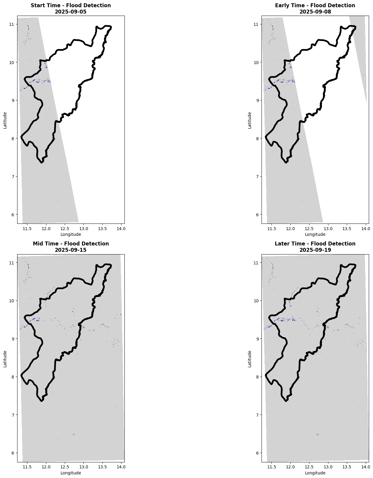
Select time slices to visualize the compositing process:
```{python}
# Get 4 Image snap-shots from STAC for visualization of concept
limg_tstart = ic_latest.isel(time=0)
limg_tearly = ic_latest.isel(time=3)
limg_tmid = ic_latest.isel(time=10)
limg_tlater = ic_latest.isel(time=14)
```
Pre-compute images for easier plot development.
```{python}
# | cache: true
# | cache-comments: "Cache computed images to avoid recomputation on plot tweaks"
# this will take a couple minutes

img_tstart = limg_tstart.compute()
img_tearly = limg_tearly.compute()
img_tmid = limg_tmid.compute()
img_tlater = limg_tlater.compute()
```
### Visualize
Plot time slices showing how flood coverage evolves and geographic gaps get filled over time. In reality we'd be doing this from the start of the historical record so we'd only see any geographic gaps in the first 2 weeks of the historical record.
```{python}
# Define colors for flood data visualization
colors = ["lightgrey", "darkblue", "white"]  # 0=no flood, 1=flood, 255=nodata

# compute_start = time.time()
cmap = ListedColormap(colors)
bounds = [0, 0.5, 1.5, 255.5]
norm = BoundaryNorm(bounds, cmap.N)

# Create 2x2 subplot grid
fig, ((ax1, ax2), (ax3, ax4)) = plt.subplots(2, 2, figsize=(20, 16))

# Define image data and metadata for loop processing
images_data = [
    {"img": img_tstart, "ax": ax1, "title": "Start Time - Flood Detection"},
    {"img": img_tearly, "ax": ax2, "title": "Early Time - Flood Detection"},
    {"img": img_tmid, "ax": ax3, "title": "Mid Time - Flood Detection"},
    {"img": img_tlater, "ax": ax4, "title": "Later Time - Flood Detection"},
]

# Process all images in a loop to avoid code repetition
processed_data = []
for i, img_info in enumerate(images_data):
    img_data = img_info["img"]
    ax = img_info["ax"]
    title = img_info["title"]

    # Process data (handle NaN and downsample)
    data_clean = np.where(np.isnan(img_data), 255, img_data)
    data_clean = data_clean[::8, ::8]  # Downsample for speed
    processed_data.append(data_clean)

    # Get extent from the xarray data
    extent = [
        img_data.x.min().item(),
        img_data.x.max().item(),
        img_data.y.min().item(),
        img_data.y.max().item(),
    ]

    # Plot the image
    im = ax.imshow(
        data_clean,
        cmap=cmap,
        norm=norm,
        interpolation="nearest",
        origin="upper",
        extent=extent,
    )

    # Add Adamawa boundary
    gdf_aoi.boundary.plot(ax=ax, color="black", linewidth=4, alpha=1.0)

    # Get the actual date from the image for the title
    img_date = img_data.time.values
    # Show just the date since we're now working with daily data
    date_str = str(img_date)[:10]  # Extract YYYY-MM-DD format

    # Set title with date and labels
    ax.set_title(f"{title}\n{date_str}", fontsize=12, fontweight="bold")
    ax.set_xlabel("Longitude")
    ax.set_ylabel("Latitude")

# total_compute = time.time() - compute_start
# print(f"✅ 2x2 flood detection plots completed in {total_compute:.1f} seconds")
for i, data in enumerate(processed_data):
    img_name = ["Start", "Early", "Mid", "Later"][i]
    print(f"{img_name} plot: {data.size:,} pixels rendered")

plt.tight_layout()
plt.show()
# Remove 'fig' to prevent duplicate display
```