# Forecast vs Retrospective Magnitudes {#sec-forecast-vs-retro}
```{python}
#| echo: false
import sys
from pathlib import Path
repo_root = str(Path.cwd().parent)
if repo_root not in sys.path:
sys.path.insert(0, repo_root)
```
The published GEOGloWS return-period thresholds are fitted to the retrospective simulation alone (`s3://geoglows-v2/retrospective/return-periods.zarr`, Log-Pearson III on retro annual maxima). For an AA trigger framework that runs against the **forecast** in real time, the question is whether the forecast magnitudes are well-calibrated by the retrospective-derived thresholds. The answer turns out to be no.
Without a multi-year reforecast archive we cannot calibrate trigger thresholds against forecast skill the way GloFAS allows. But the live forecast archive does extend ~22 months back (2024-07-01 to today), enough to compare day-by-day forecast magnitudes against the retrospective on the same valid date. Doing so reveals a systematic, lead-time-independent magnitude bias.
## Method
For 667 daily forecast issue dates across 2024-07-01 to 2026-04-29 (one date failed to fetch), we extracted the day-0 to day-14 forecast (52-member ensemble mean) for each of our two reaches directly from the per-date Zarr stores. Each (issue_date, lead_day) pair is then matched to the retrospective discharge on the corresponding **valid date** (= issue_date + lead_day), and we compare them.
```{python}
#| eval: true
import numpy as np
import ocha_stratus as stratus
import pandas as pd

from src.constants import BLOB_PREFIX, BLOB_STAGE, STATIONS
from src.utils import load_geoglows_retro

df = stratus.load_parquet_from_blob(
    f"{BLOB_PREFIX}/forecast_lead_times_v2.parquet", stage=BLOB_STAGE
)
df["forecast_date"] = pd.to_datetime(df["forecast_date"])
df["valid_date"] = df["forecast_date"] + pd.to_timedelta(df["lead_day"], unit="D")
rid_to_name = {s.geoglows_river_id: s.name for s in STATIONS.values()}
df["station"] = df["river_id"].map(rid_to_name)

retros = {
    s.name: load_geoglows_retro(s.geoglows_river_id)["discharge"]
    for s in STATIONS.values()
}
df["retro"] = df.apply(
    lambda r: retros[r["station"]].get(r["valid_date"], np.nan), axis=1
)
df = df.dropna(subset=["retro"]).copy()
df["ratio"] = df["fc_avg"] / df["retro"]
df["bias"] = df["fc_avg"] - df["retro"]

print(f"Rows: {len(df):,}")
print(f"Date range: {df.forecast_date.min().date()} to {df.forecast_date.max().date()}")
print(f"Stations × lead days: {df.station.nunique()} × {df.lead_day.nunique()}")
```
## The bias is constant across lead times (Chatara)
```{python}
#| eval: true
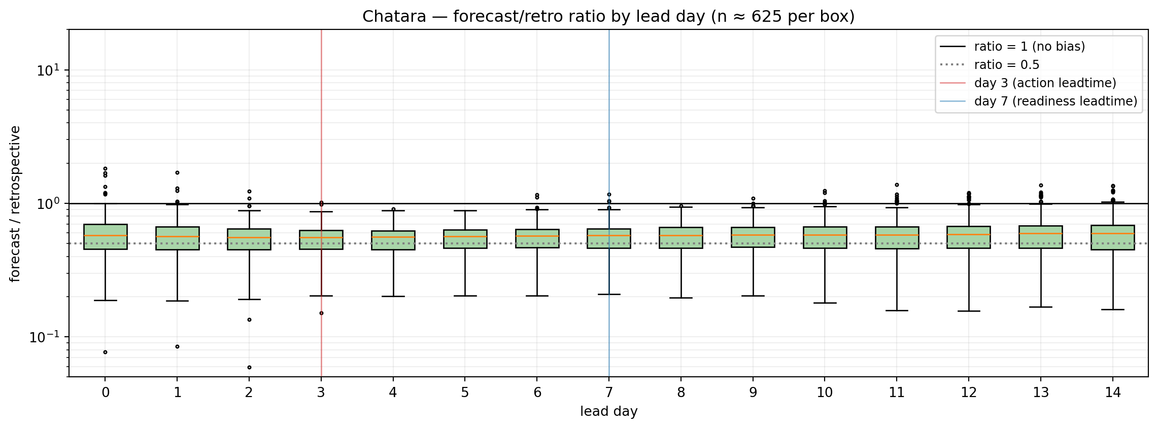
#| fig-cap: "Chatara: forecast/retrospective ratio by lead day. Median ~0.55 at every lead time, including the 3-day (action) and 7-day (readiness) leadtimes used by the AA framework. Lead-time choice does not change the bias."
import matplotlib.pyplot as plt

fig, ax = plt.subplots(figsize=(12, 4.5))
sub = df[df.station == "Chatara"].copy()
sub = sub[(sub.retro > 0) & (sub.fc_avg > 0)]
groups = [sub[sub.lead_day == ld].ratio.values for ld in range(15)]

bp = ax.boxplot(groups, positions=range(15), widths=0.6,
                patch_artist=True, showfliers=True,
                flierprops=dict(markersize=2))
for patch in bp["boxes"]:
    patch.set_facecolor("#a8d5a8")
ax.axhline(1, color="k", lw=1, label="ratio = 1 (no bias)")
ax.axhline(0.5, color="gray", ls=":", label="ratio = 0.5")
ax.axvline(3, color="#d62728", ls="-", lw=1, alpha=0.5, label="day 3 (action leadtime)")
ax.axvline(7, color="#1f77b4", ls="-", lw=1, alpha=0.5, label="day 7 (readiness leadtime)")
ax.set_yscale("log")
ax.set_ylim(0.05, 20)
ax.set_xticks(range(15))
ax.set_xlabel("lead day")
ax.set_ylabel("forecast / retrospective")
ax.set_title("Chatara — forecast/retro ratio by lead day (n ≈ 625 per box)")
ax.legend(fontsize=9, loc="upper right")
ax.grid(alpha=0.2, which="both")
plt.tight_layout()
plt.show()
```
The box centers sit at ~0.55 from day 0 to day 14. Box widths grow slightly with lead time (forecast uncertainty), but the central tendency does not move. The forecast at the AA action leadtime (day 3) and readiness leadtime (day 7) is biased identically to day 0.
## The forecast distribution sits on the 2:1 line at all leadtimes
```{python}
#| eval: true
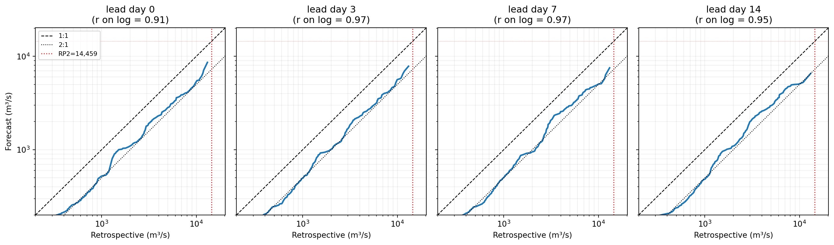
#| fig-cap: "Chatara — Q-Q plots of forecast vs retrospective at lead days 0, 3, 7, 14. The forecast distribution lies on the 2:1 line (forecast = retro/2) at every lead time. The published RP2 (14,459 m³/s) is never reached on the ensemble mean — the highest ensemble-mean value in the archive is ~9,000 m³/s."
rid = 441135650
rp = stratus.load_parquet_from_blob(
    f"{BLOB_PREFIX}/geoglows_return_periods_{rid}.parquet", stage=BLOB_STAGE
).iloc[:, 0].to_dict()

fig, axes = plt.subplots(1, 4, figsize=(15, 4.5), sharex=True, sharey=True)
qs = np.linspace(0.01, 0.999, 200)
for ax, ld in zip(axes, [0, 3, 7, 14]):
    sub = df[(df.station == "Chatara") & (df.lead_day == ld)]
    paired = sub[["retro", "fc_avg"]].dropna()
    retro_q = np.quantile(paired.retro, qs)
    fc_q = np.quantile(paired.fc_avg, qs)
    r = np.corrcoef(np.log(paired.retro), np.log(paired.fc_avg))[0, 1]

    ax.plot(retro_q, fc_q, "-", c="#1f77b4", lw=2)
    lo, hi = 200, max(retro_q.max(), rp[5]) * 1.1
    ax.plot([lo, hi], [lo, hi], "k--", lw=1, label="1:1")
    ax.plot([lo, hi], [lo / 2, hi / 2], "k:", lw=1, label="2:1")
    ax.axvline(rp[2], color="#d62728", ls=":", lw=1.2,
               label=f"RP2={rp[2]:,.0f}")
    ax.axhline(rp[2], color="#d62728", ls=":", lw=0.6, alpha=0.5)
    ax.set_xscale("log"); ax.set_yscale("log")
    ax.set_xlim(lo, hi); ax.set_ylim(lo, hi)
    ax.set_xlabel("Retrospective (m³/s)")
    ax.set_title(f"lead day {ld}\n(r on log = {r:.2f})")
    ax.grid(alpha=0.2, which="both")
    if ld == 0:
        ax.set_ylabel("Forecast (m³/s)")
        ax.legend(fontsize=8, loc="upper left")
plt.tight_layout()
plt.show()
```
Q-Q correlation on log-discharge is **0.91 at lead 0**, **0.97 at lead 3 and 7**, and **0.95 at lead 14** — the forecast tracks the retrospective shape extremely well. The bias is purely in magnitude. The forecast curve sits on the 2:1 line (forecast ≈ retro / 2) across the full distribution at every lead time. The published RP2 of 14,459 m³/s is never reached on the ensemble mean: the highest fc_avg across all 667 issue dates × 15 lead days at Chatara is 9,016 m³/s. Individual ensemble members do occasionally exceed RP2 — 23 of 10,005 (date, lead_day) cells contain at least one such member — but no (date, lead_day) cell has an ensemble-mean exceedance.
## What this means for the AA framework
If we used GEOGloWS forecasts as a real-time trigger and applied the published retrospective-derived RP thresholds:
- **At Chatara, an ensemble-mean trigger would never fire** at RP2, regardless of which lead time we used. A "any-member exceeds RP2" trigger fires on 23 of 10,005 (date, lead_day) cells (~0.23%), most clustered around the 2024-07 monsoon peak.
- **At any AA-relevant lead time** (day 3 action, day 7 readiness), the bias is the same as at day 0. We cannot pick a better lead time to escape the bias.
To use the GEOGloWS forecast as an operational trigger, we would need to **calibrate forecast-specific thresholds from the forecast archive itself**, not from the retrospective. With ~22 months of archive that's still too short for stable rare-event RP estimation (a 22-month archive contains zero or one RP2 events by definition), so the calibration would be weak even if attempted.
The published RPs reflect what the *retrospective simulation* thinks happened over 1940–present. They do not reflect what the *operational forecast* produces. Using them as forecast triggers is a category error.
## Why this is the binding constraint on using GEOGloWS for the AA framework
The framework needs:
1. **Hindcasts (multi-year reforecasts)** to calibrate lead-time-dependent skill metrics (exceedance probability at fixed leadtimes). GEOGloWS does not provide these.
2. **Calibrated thresholds** that reflect the forecast distribution, not just the retrospective. GEOGloWS's published RPs are retrospective-only.
The first gap is structural — GEOGloWS does not publish a multi-year reforecast archive (see Chapter 1). The second gap is what this chapter documents empirically: the forecast and retrospective produce systematically different magnitudes for the same days, and the published thresholds are calibrated to one and applied to the other. Together these gaps mean a GEOGloWS-based AA trigger cannot be calibrated to fire at the intended frequency without independent data we do not have.