# Threshold Comparison
```{python}
#| echo: false
import sys
from pathlib import Path
repo_root = str(Path.cwd().parent)
if repo_root not in sys.path:
sys.path.insert(0, repo_root)
```
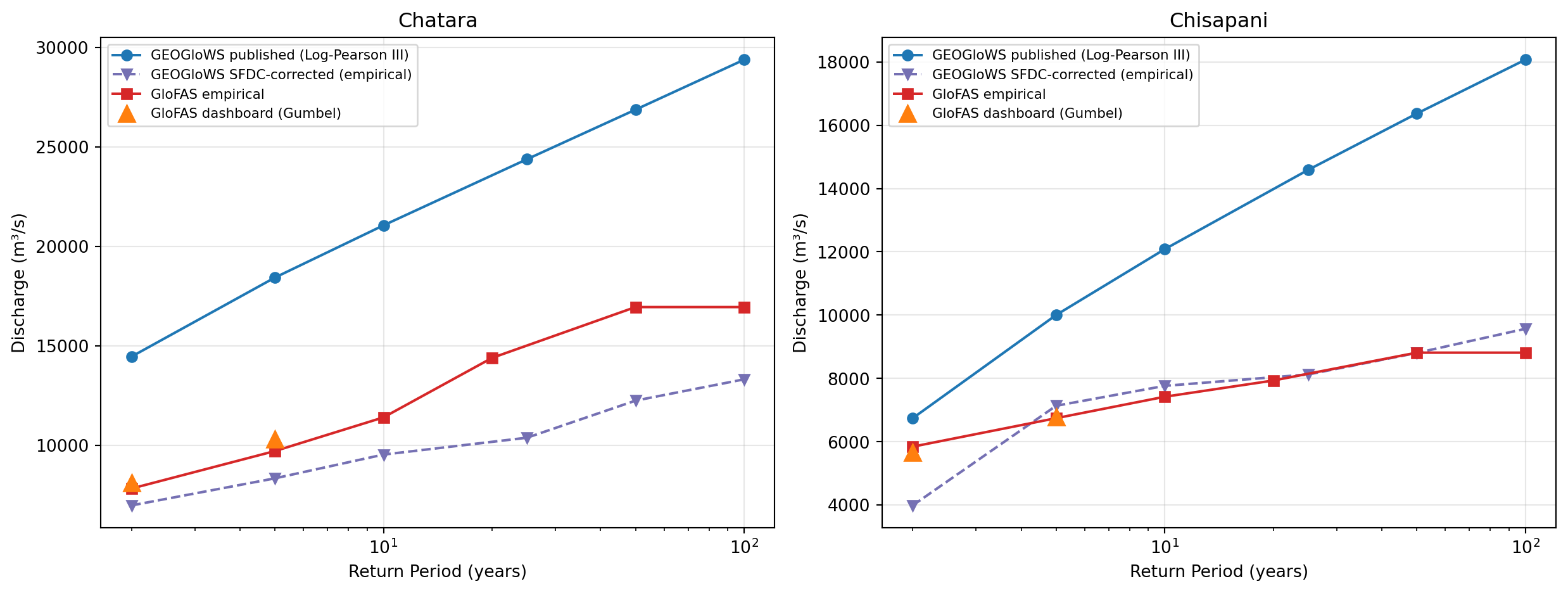
Return-period thresholds define what counts as a "significant" flood event in the AA framework. Different sources fit different distributions to different record lengths, so the threshold values diverge — sometimes a lot. This chapter compares them and asks whether GEOGloWS's built-in SFDC bias correction narrows the gap with GloFAS.
## Sources and Methods
| Source | Period | Distribution | Notes |
|--------|--------|-------------|-------|
| GloFAS Copernicus dashboard | 1979–present | Gumbel Type I | Fitted to reanalysis annual maxima |
| GloFAS empirical | 1979–2023 | Empirical quantile | Ranked annual maxima (notebook 01.0) |
| GEOGloWS published | 1940–present | Log-Pearson III | Pre-computed via `geoglows.data.return_periods` |
| GEOGloWS empirical (uncorrected) | 1940–present | Empirical quantile | Computed from retro daily |
| GEOGloWS empirical (SFDC corrected) | 1940–present | Empirical quantile | After `geoglows.bias.sfdc_bias_correction` |
GEOGloWS's record is 86 years vs GloFAS's 44, but the underlying hydrology also differs — RAPID is a routing-only model running on TDX-Hydro, while LISFLOOD is a calibrated full land-surface model.
## Cross-Source Comparison
```{python}
import ocha_stratus as stratus
import pandas as pd
from src.constants import BLOB_PREFIX, BLOB_STAGE, RETURN_PERIODS, STATIONS
from src.utils import (
    compute_return_levels,
    load_geoglows_retro,
    load_geoglows_retro_corrected,
)

# GloFAS empirical return levels from reanalysis (1979-2023), source: notebook 01.0
GLOFAS_EMPIRICAL = {
    "Chatara": {2: 7831, 5: 9716, 10: 11408, 20: 14396, 50: 16951, 100: 16951},
    "Chisapani": {2: 5847, 5: 6747, 10: 7424, 20: 7936, 50: 8816, 100: 8816},
}

rows = []
for key, station in STATIONS.items():
    rid = station.geoglows_river_id
    rp_pub = stratus.load_parquet_from_blob(
        f"{BLOB_PREFIX}/geoglows_return_periods_{rid}.parquet", stage=BLOB_STAGE
    ).iloc[:, 0].to_dict()
    rp_orig_emp = compute_return_levels(
        load_geoglows_retro(rid)["discharge"], RETURN_PERIODS
    )
    rp_corr_emp = compute_return_levels(
        load_geoglows_retro_corrected(rid)["discharge"], RETURN_PERIODS
    )
    glofas_emp = GLOFAS_EMPIRICAL[station.name]
    glofas_dashboard = {2: f"{station.glofas_rp2:,}", 5: f"{station.glofas_rp5:,}"}

    for rp in [2, 5, 10, 25, 50, 100]:
        rows.append({
            "Station": station.name,
            "Return Period": f"{rp}-yr",
            "GloFAS Dashboard": glofas_dashboard.get(rp, "—"),
            "GloFAS Empirical": f"{glofas_emp[rp]:,}" if rp in glofas_emp else "—",
            "GEOGloWS Published": f"{rp_pub[rp]:,.0f}",
            "GEOGloWS Empirical": f"{rp_orig_emp[rp]:,.0f}",
            "GEOGloWS SFDC-corrected": f"{rp_corr_emp[rp]:,.0f}",
        })

comparison = pd.DataFrame(rows)
comparison
```
## Visual Comparison
```{python}
import matplotlib.pyplot as plt

fig, axes = plt.subplots(1, 2, figsize=(13, 5))

for ax, (key, station) in zip(axes, STATIONS.items()):
    rid = station.geoglows_river_id

    rp_pub = stratus.load_parquet_from_blob(
        f"{BLOB_PREFIX}/geoglows_return_periods_{rid}.parquet", stage=BLOB_STAGE
    ).iloc[:, 0]
    rp_corr_emp = compute_return_levels(
        load_geoglows_retro_corrected(rid)["discharge"], RETURN_PERIODS
    )

    ax.plot(rp_pub.index, rp_pub.values, "o-",
            label="GEOGloWS published (Log-Pearson III)", color="#1f77b4")
    ax.plot(list(rp_corr_emp.keys()), list(rp_corr_emp.values()), "v--",
            label="GEOGloWS SFDC-corrected (empirical)", color="#7570b3")

    glofas_emp = GLOFAS_EMPIRICAL[station.name]
    emp_rps = sorted(glofas_emp.keys())
    ax.plot(emp_rps, [glofas_emp[r] for r in emp_rps], "s-",
            label="GloFAS empirical", color="#d62728")
    ax.plot(2, station.glofas_rp2, "^", color="#ff7f0e", markersize=10,
            label="GloFAS dashboard (Gumbel)")
    ax.plot(5, station.glofas_rp5, "^", color="#ff7f0e", markersize=10)

    ax.set_xscale("log")
    ax.set_xlabel("Return Period (years)")
    ax.set_ylabel("Discharge (m³/s)")
    ax.set_title(station.name)
    ax.legend(fontsize=8)
    ax.grid(True, alpha=0.3)

plt.tight_layout()
plt.show()
```
## What the numbers say
**Uncorrected, GEOGloWS RPs are higher than GloFAS:**
- **Chatara RP2**: 14,459 (GEO) vs 8,113 (GloFAS dashboard) — **+78%**
- **Chatara RP5**: 18,433 vs 10,306 — **+79%**
- **Chisapani RP2**: 6,745 vs 5,664 — **+19%**
- **Chisapani RP5**: 10,005 vs 6,797 — **+47%**
**SFDC bias correction overshoots the gap and pushes most GEOGloWS RPs *below* GloFAS:**
- **Chatara RP2**: 14,459 → 6,983 (now 14% below GloFAS dashboard)
- **Chatara RP5**: 18,433 → 8,345 (now 19% below)
- **Chisapani RP2**: 6,745 → 3,992 (now 30% below)
- **Chisapani RP5**: 10,005 → 7,139 (5% above)
In other words, SFDC does not gently align GEOGloWS with GloFAS — it deflates the entire distribution. The Chatara mean drops from 2,258 to 1,585 m³/s and the maximum is roughly halved (27,064 → 13,319 m³/s). That magnitude shift carries through to the empirical RP estimates.
## Why uncorrected GEOGloWS reads higher
Several factors push the published Log-Pearson III estimates above GloFAS:
1. **Distribution choice**: Log-Pearson III has a heavier tail than Gumbel.
2. **Record length**: 86 years (GEOGloWS) vs 44 (GloFAS). The longer record can sample rarer events. GEOGloWS's largest annual maxes for Chisapani fall in 1947, 1948, 1951, 1957–59, 1971, and 1974 — entirely outside the GloFAS window.
3. **Model differences**: RAPID routes ECMWF/ERA5 runoff through a vector network with no calibration step; LISFLOOD is a full land-surface model calibrated against ~2,000+ gauges.
4. **River delineation**: TDX-Hydro reach areas are not guaranteed to match GloFAS grid-cell drainage.
## Bias correction: what it does and does not do
`geoglows.bias` exposes three methods. Only one is usable here:
| Method | Requires observed discharge? | Status |
|--------|------------------------------|--------|
| `correct_historical()` | Yes | Blocked: DHM provides water level, not discharge |
| `correct_forecast()` | Yes | Same blocker |
| `sfdc_bias_correction()` | No (uses pre-computed SABER scalars) | Applied here |
SFDC works by looking up pre-computed scalar correction factors for each month and percentile of the simulated flow-duration curve and rescaling the simulation accordingly. The correction is global — derived from the SABER reference dataset — and does not learn from local observations.
The threshold-level finding above is that SFDC consistently *deflates* both stations. Whether that helps the actual use case (detecting observed flood events) is the question for @sec-event-detection.
## Window sensitivity: published RPs are not stable across the record
The published GEOGloWS RPs are fitted to the full 1940–present retrospective. If the model behaves differently in the early period than in the validation window we have DHM data for, the published threshold is biased relative to what would be empirically reasonable for the validation period.
```{python}
windows = []
for key, station in STATIONS.items():
    rid = station.geoglows_river_id
    series = load_geoglows_retro(rid)["discharge"]
    pub = stratus.load_parquet_from_blob(
        f"{BLOB_PREFIX}/geoglows_return_periods_{rid}.parquet", stage=BLOB_STAGE
    ).iloc[:, 0].to_dict()
    full = compute_return_levels(series, [2, 5])
    val = compute_return_levels(
        series[(series.index.year >= 1985) & (series.index.year <= 2014)], [2, 5]
    )
    pre = compute_return_levels(series[series.index.year < 1985], [2, 5])
    for rp in [2, 5]:
        windows.append({
            "Station": station.name,
            "RP": f"{rp}-yr",
            "Published (LP3, full)": f"{pub[rp]:,.0f}",
            "Empirical (full 1940–present)": f"{full[rp]:,.0f}",
            "Empirical (1985–2014, validation)": f"{val[rp]:,.0f}",
            "Empirical (pre-1985)": f"{pre[rp]:,.0f}",
        })
pd.DataFrame(windows)
```
For Chatara the windows agree to within ~7%. For **Chisapani the validation-window RP2 is 5,288 vs 6,745 published — about 22% lower**. The pre-1985 era contains the largest GEOGloWS Karnali peaks (1947, 1948, 1951, 1957–59) that pull the LP3 fit upward.
This matters: if you used the published RP2 as a trigger but the model's 1985-onward statistics don't support it, you'd be using a threshold the modern record rarely produces. Whether that effect is large enough to matter for detection is tested in @sec-event-detection — applying the validation-window RP2 to the validation slice, the answer is "marginally for Chatara, not at all for Chisapani."
## Implication
RP-based triggers are normalized to the data source by construction: applying each source's RP2 to its own record fires at roughly the same long-run frequency (~1 in 2 years), regardless of whether that threshold is 5,664 or 14,459 m³/s. The magnitude divergence above does not change the *number* of triggers, only the threshold value at which each source fires.
What the magnitude divergence tells us is how differently each source represents the basin's flood regime. SFDC correction does not split the difference; it overshoots, putting most GEOGloWS RPs below GloFAS. Whether any of these definitions actually fires on the right days — the events DHM observed — is the question for @sec-event-detection. The next chapter first looks at the time series and seasonal cycle to see whether the sources at least agree about when monsoon flow peaks and how big it gets.