They are anchored beside the passage each one concerns. Nothing in the trigger design has been changed: the configuration, the numbers and the figures are exactly as generated. What has been corrected is text that contradicted the data, plus the broken provider switch; supporting evidence has been folded into collapsible blocks.
- R1: the “7 of 8” headline rests on a lookahead in the benchmark
- R2: every published lag is wrong; correlations understated
- R3: three provider sets were really two
- R4: the Juba leg never decides anything
- R5: the per-window search does not beat an un-searched rule
- R6: one model per window is defensible; mixing gains nothing
- R7: the seven-point set cannot be reduced, and two points are unverifiable
- R8: excluding GEOGloWS introduces the one false activation
- R9: the two lead bands overlap at lead 7
- R10: ten of fourteen activations have no readiness phase
- R11: 1999–2001 unassessable but still in every denominator
- R12: some benchmark levels rest on ten annual maxima
One label to keep in mind while reading: the benchmark that decides which years count as severe was refitted after the figures below were generated. On the current fit there are seven severe years and the trigger catches all of them; the older figures and prose count 2008 as an eighth severe year and the one miss. The activation years are identical either way. See the benchmark note under Skill scores.
The mechanism at a glance
Across 1999–2023 the envelope is identical to the Shabelle river on its own: there is no year in which the Juba activates and the Shabelle does not. Per-river rates are 1-in-4.3 (Juba) against 1-in-3.2 (Shabelle), so the equal-probability-per-river goal is not met. Both Gu windows also run on Google and activate in the same four years (2013, 2016, 2018, 2020), so the Gu half of the mechanism is effectively a single trigger counted twice.
Four river-season windows, each running on one forecast source rather than a mixture. Inside a window, every monitored point's flow is compared with its own return-period threshold and the window activates when enough points are over their thresholds on the same day. A season where the points cross on different days does not count. This rarely matters in practice: flood flows stay high for weeks, and in every past activation the points crossed within 0 to 5 days of each other, upstream gauges first (see "How far apart do the points cross?" below). The required count is set between two and one fewer than the river's points: no single gauge can release the money, and no single quiet or broken gauge can block it. More points crossing than required, including all of them, simply activates the window.
All seven reporting-era points are monitored: four on the Juba (Luuq, Dollow, Bardheere, Bualle) and three on the Shabelle (Belet Weyne, Bulo Burti, Jowhar). No threshold, on either leg, sits below 1-in-3. The four windows together are called the envelope: the full amount is released whenever any one of them activates, so the envelope is what the budget is sized on and what the 1-in-3 ceiling applies to.
Restricting to the five gauges that still report would leave the Juba with only Luuq and Dollow, so the only available rule is 2 of 2, which is unanimous and forbidden by this design's own “never all of them” constraint, and it adds a false activation in 2015, moving the envelope to 1-in-2.9. Bardheere and Bualle are therefore what make a non-unanimous Juba rule possible. The cost is that an activation driven by those two points can never again be verified against an observation: Bardheere's record ends 2023-11-30 and Bualle's 2024-03-14.
| window | action trigger (leads 1-7 d) | leg RP | readiness (leads 8-12 d, same reanalysis levels, RP capped at 1-in-5) | readiness RP (2003-2023) |
|---|---|---|---|---|
| Juba Gu | Google GRRR: 3 of 4 points over their 1-in-5-yr thresholds | 6.5 yr | GloFAS v4 ens-median: 3 of 4 over 1-in-5-yr | 22.0 yr |
| Juba Deyr | GloFAS v5: 3 of 4 points over their 1-in-4-yr thresholds | 13.0 yr | GloFAS v4 ens-median: 3 of 4 over 1-in-4-yr | 11.0 yr |
| Shabelle Gu | Google GRRR: 2 of 3 points over their 1-in-6-yr thresholds | 6.5 yr | GloFAS v4 ens-median: 2 of 3 over 1-in-5-yr | 7.3 yr |
| Shabelle Deyr | GloFAS v5: 2 of 3 points over their 1-in-5-yr thresholds | 6.5 yr | GloFAS v4 ens-median: 2 of 3 over 1-in-5-yr | 11.0 yr |
How the two rivers behave together
The Shabelle activates more often: 8 of 25 years (1-in-3.2) against the Juba's 6 (1-in-4.3). There is no year in which the Juba activates and the Shabelle does not; the Shabelle alone adds 2014 and 2019. Six activations fall in the same season on both rivers, and in all six the Juba reaches its thresholds first, by 1 to 24 days:
| season | Juba crosses | Shabelle crosses | lead |
|---|---|---|---|
| Gu 2013 | 12 Apr | 6 May | Juba first, 24 d |
| Gu 2016 | 7 May | 12 May | Juba first, 5 d |
| Gu 2018 | 20 Apr | 5 May | Juba first, 15 d |
| Gu 2020 | 29 Apr | 30 Apr | Juba first, 1 d |
| Deyr 2006 | 29 Oct | 2 Nov | Juba first, 4 d |
| Deyr 2023 | 29 Oct | 10 Nov | Juba first, 12 d |
So the Juba never adds an activation year (review note R4), but in every shared season it crosses first. Since either window releases the full amount, the Juba sets the response date in those six years; the Shabelle activates more often and adds the years the Juba misses.
Each gauge's return level is fitted on 2000–2026 while crossings are counted only within 1999–2023, so three years of post-window data enter the labels. That is what makes 2008 severe: Luuq's Deyr 1-in-5 level is 5.831 m fitted through 2026 but 5.869 m fitted through 2023, and the 2008 peak is 5.840 m, a 9 mm margin on a level that moves 38 mm purely from adding future years. Fit strictly to the backtest window and the severe set is 7, not 8, and this configuration catches 7 of 7. The much-discussed “miss in 2008” is an artifact of the asymmetry, since trigger thresholds are fitted strictly on 1999–2023. Corrected in scripts/envelope_search.py on 2026-09-18 (gauge levels fitted 2000–2023, closed at the last backtest year); the corrected numbers are used on the design comparison page, in the trigger summary and in the sections of this page added from 7 September onwards, while the earlier figures and tables on this page still count 2008 as an eighth severe year.
The obvious answer is to debias, and that is what cannot be done yet: the GEOGloWS forecast archive begins in July 2024, roughly two years, which is neither enough to refit thresholds on the forecast climatology (this design asks about twelve years for a 1-in-3) nor enough to validate a flow-duration-curve correction against anything. The team's Nepal technical note records the same result: SFDC did not rescue event detection there. The working group therefore leaned to excluding GEOGloWS on 2026-08-22 and adopted that on 2026-08-28. It stays in this view as a comparison, and stays a candidate for reinstatement once two or three Gu and Deyr seasons of its forecasts exist.
- It agrees with the impact record on the big riverine years. 2006, 2018, 2019, 2020 and 2023 are all severe under the rule. Ranked on raw totals from EM-DAT, the international disaster database, though, the third-costliest flood year is 2015 (916,000 affected), which the rule does not call a flood at all, correctly, since that event was in Galgaduud, Mudug and Nugal rather than on either river. The agreement holds only once EM-DAT is filtered to Juba and Shabelle events.
- 1999 to 2001 cannot be assessed. The Juba had no gauge reporting and the Shabelle only one, so no consensus is possible and those years read as quiet rather than as unknown. Nothing activates before 2005, so no year is wrongly scored as a miss, but the benchmark effectively starts in 2002.
- 2021 is a genuine gap. EM-DAT records 400,000 people affected, yet only Bardheere on the Juba and Belet Weyne on the Shabelle crossed, so the rule reads no flood. Belet Weyne's peak that year sits exactly at bank full (8.30 m), where the gauge record is censored and the true level is unknown, so consensus can be understated in exactly the years that matter most.
- 2016 is the reverse case. Three of the four Juba gauges and all three Shabelle gauges crossed their levels in Gu, but EM-DAT records nobody affected. Gauge levels and recorded impact are not the same measurement.
No window can reach two reporting gauges in those years, so they are scored as “no flood” rather than as unknown, while 25 years remains the denominator for every return period quoted on this page. The assessable record is effectively 22 years. The same mechanism silently affects Shabelle Deyr in 2000 and 2001, where Jowhar was the only reporting gauge and did cross its level, and Juba Gu in 2005–2006.
The stated ceiling of “a quarter of the record” is applied to the forecast thresholds but not to the benchmark. Dollow has 10 Deyr annual maxima after 2000 and is still assigned a 1-in-5 level; Bualle has 16. Since a single gauge crossing decides whether the two-gauge rule is met, a level interpolated from ten values can decide whether a year counts as a flood at all.
What happens if Google Flood Hub goes away
Use the provider switch above. Removing Google returns the configuration to the all-providers one: GEOGloWS takes Juba Gu and GloFAS v5 takes the other three windows. The envelope stays at 1-in-3.2 (8 of 25 years) with the same severe-year coverage, and it loses the 2013 activation, so on the calibration record dropping Google costs nothing measurable. The catch is that the replacement is GEOGloWS, the one model whose thresholds cannot yet be fitted on its own forecasts, so the fallback is weaker operationally than it looks on the backtest.
The “without Google” configuration is numerically identical to “all providers”, because when GEOGloWS is allowed to compete Google never wins a window. The third switch state has been removed, and the two competing switch controllers that were both live on the page (which corrupted the default view once you clicked) have been reduced to one.
The decision was taken by the working group (leaning this way on Friday 2026-08-22, adopted 2026-08-28) and the reasoning is sound; the callout above gives the quantified version. The cost should be recorded alongside it: the all-providers configuration activates in 8 years with no activation outside the benchmark, whereas the adopted one activates in the same number of years but activates in 2013, a year the two-gauge benchmark does not call a flood. Trading one false activation for a model that can actually be operated is a defensible trade; it is just better made explicitly.

- One source per river-season window, never a mixture: requested by WFP, who raised concerns about mixing models inside a window. Tested against the alternative it costs nothing measurable (review note R6).
- GEOGloWS excluded: working group decision, leaning that way 2026-08-22 and adopted 2026-08-28, because its forecasts run below its own retrospective and its two-year forecast archive is too short either to refit thresholds on or to validate a debias against.
- The envelope activates no more often than 1-in-3: directive of 2026-08-27, applied to the union of the four windows rather than to each window.
How the model was chosen, one per river and season
Applying one model, one return period and one vote count uniformly to all four windows: Google GRRR, 1-in-6, 3 of 4 reproduces the adopted result exactly (8 activations, 1-in-3.2, every severe year caught, the 2013 false alarm). GloFAS v5, 1-in-5, 3 of 4 gives 9 activations at 1-in-2.9 with the same severe-year coverage and zero activations outside the benchmark. The roughly 41,000 admissible per-window combinations recover nothing a one-line rule does not. This is consistent with the page's own statement that many assignments tie, but it is stronger: the per-window freedom is not adding measurable value. Partly answered by the swap test added 1 September, which I have reproduced and which holds: at the adopted return periods and vote counts, neither model alone can carry all four windows without breaching the 1-in-3 ceiling, since Google everywhere lands at 1-in-2.6 and GloFAS v5 everywhere at 1-in-2.9, so the mixed
assignment is doing real work, and the Deyr case for GloFAS v5 rests on the Juba (Google brings
three activations outside the benchmark there; on the Shabelle both models miss the 2020 severe
year at 1-in-5). Those conclusions are unchanged on the corrected benchmark. What remains of this note is narrower: the swap test holds the thresholds fixed at the adopted values, so it shows the assignment is defensible given those settings, not that the configuration as a whole beats a simpler one. A uniform rule at different settings, Google GRRR at 1-in-6 with 3 of 4 in every window, still reproduces the adopted envelope exactly. Both are true: the assignment is justified, and the tuning around it is not what produces the result.
One source per river and season, so four choices. Four steps:
The constraint is a stakeholder requirement, not a data-driven one: WFP raised concerns about mixing models within a window. On this record it costs nothing measurable. Allowing every model to compete at every point inside a window (a mixed consensus over the same seven points) reaches the same severe-year coverage at 1-in-3.7 that the best single-model configuration reaches at 1-in-3.2. Mixing buys no additional severe year, so the requirement can be honoured without giving anything up, and it simplifies operations, since one model per window means one threshold transfer to validate rather than several.
- Build the candidate rules. For a window and a candidate model, put a threshold at every one of the river's points, taken from that model's own annual maxima (1-in-3 to 1-in-6). The window activates in a year when at least N points cross in that season.
- Score the envelope, not the window. The money is released when any of the four windows activates, so candidates are judged on that union: how often it activates, how many of the severe years it catches, and how often it activates in a year with no recorded flood.
- Apply the constraints. Thresholds never below 1-in-3 nor above a quarter of the record; all seven points monitored; at least two must agree but never all of them; every window must activate at least twice in 25 years.
- Pick. Nearest 1-in-3 overall with the most severe years caught. Ties break on fewer no-flood activations, then on tracking correlation.

The per-point tracking numbers behind the choice (ρ and best lag of each model against the river's reference gauge):
The best-lag search shifts the gauge series by row position after filtering to season months, so any non-zero lag pulls rows from the adjacent year and always scores worse than lag 0. The result is that 46 of the 56 cells below report a lag of exactly 0, including Bualle against the Luuq reference gauge some 450 km upstream. Recomputed with a calendar-day shift, Belet Weyne against GloFAS v4 in Deyr peaks at +22 days with ρ 0.78, not at 0 days with ρ 0.67. Because tracking correlation is the final tie-break between models, that tie-break is currently running on a corrupted statistic. Corrected on branch fix/corrected-benchmark-and-lag (not merged, and this page is unchanged); the corrected numbers are used on the design comparison page.
Per-station selection detail (ρ / lag per model, all four windows)
Why the models perform the way they do
The main difference between the models is magnitude. Each reproduces the shape of the flood tail reasonably well, but over- or under-estimates its size by a roughly constant factor.

- GEOGloWS runs 3.8 to 10 times too high on the Shabelle and at Luuq, at every return period. It ranks wet and dry years reasonably well, but its absolute discharge is far off.
- GloFAS v5 is the closest to the observations: 1.12 to 1.25 at Belet Weyne, 1.24 to 1.42 at Bulo Burti, 0.83 to 0.87 at Luuq. Its predecessor v4 ran 1.7 to 3.8 times too high, and v5 improves the daily rank correlation at the same time (Belet Weyne 0.65 to 0.77), so the gain is not just a rescaling. v4 is not a candidate for the action leg. It appears as the readiness leg's reforecast, the sole archive covering the 8-to-12-day readiness leads (the archive covers leads 8 to 12), and in the skill scores and the forecast-issue comparisons, because it is the model that runs live.
- Google GRRR is close on the Shabelle (0.78 to 1.11) and runs about 0.4 times observed at Luuq.
- Bardheere disagrees with everything (0.14 to 1.53 across the candidates). That points to problems with the gauge record there, not with the models.
The same comparison at the level the trigger operates: each window's vote rule, 3 of 4 points on the Juba and 2 of 3 on the Shabelle at the adopted return periods, with each model swapped in. POD (probability of detection) counts severe years caught, the objective the envelope is sized on. FAR (false alarm ratio) counts activations with no 1-in-3 flood behind them. Skill scores below defines both in full, with the rest of the contingency table:

The same test on the forecasts the trigger would actually run on, at action leads of 1 to 7 days. GloFAS v5 has no reforecast, so GloFAS is represented by the v4 ensemble median, its only lead-time archive; GEOGloWS has no archive before July 2024 and cannot be scored:

- On severe years, Gu is a tie. Both models catch 2018 and 2020 on the Juba and 2016 and 2020 on the Shabelle, and both miss Gu 2023.
- Deyr on Google is worse on the Juba: three activations outside the benchmark (2013, 2015, 2019) against none for GloFAS v5, with both models missing 2014. On the Shabelle the two models catch the same four severe years and both miss 2020 at 1-in-5; Google adds 2008, a 1-in-3 flood year. GloFAS v5's Deyr record has no activation outside the benchmark.
- GloFAS v5 alone cannot meet the 1-in-3 ceiling. No v5-only configuration reaches 8 activations, and its nearest envelope activates once every 2.9 years. Some windows therefore have to run on Google, and Gu is where the swap costs nothing.
- Google is the only model with forecast-side evidence. Its reforecast (2016-2023) shows event skill at leads 1 to 7 on the Shabelle; the only GloFAS lead-time archive (v4) scores near chance there. GloFAS v5 has no reforecast. It keeps Deyr on its reanalysis record; its thresholds carry over unchanged once GloFAS ships a v5 forecast, and until then the Deyr windows are monitored on the v4 forecast with levels refit on v4's own climatology at the same return periods.
GEOGloWS maps the RP3 events least well of the models shown. It reaches 0.30 at Belet Weyne against GloFAS v5's 0.60, 0.11 at Luuq against 0.44 for both v5 and Google, and 0.25 at Bardheere, and it pairs those misses with the worst false-alarm rates on the board: 0.88 at Luuq and Bardheere, 0.62 at Belet Weyne. It is not uniformly worst: it ties v5 at Bulo Burti (0.44) and reaches 0.67 at Dollow, where every model does well. These detection numbers, together with the threshold problem described above, are why it is left out of the adopted design.
GloFAS v5 is best or joint-best at six of the seven gauges and has the cleanest false-alarm record (0.14 at Belet Weyne, 0.40 at Dollow), which is why it carries both Deyr windows. Its weakest gauge is Bualle, where it catches 0.29 against 0.43 for the others. Google matches v5 at Dollow (1.00), Luuq (0.44) and Bardheere (0.50) and is the only model with a usable forecast archive on the Shabelle, which is why it carries Gu.
No model does well at Jowhar (0.10 to 0.20, false alarms 0.71 and up): off-takes and marsh hydraulics decouple the local level from upstream discharge. Requiring two gauges keeps it from deciding anything on its own.
This shapes the mechanism in three ways. Thresholds are set on return periods, not on absolute discharge: with a flat tail ratio, matching frequency corrects the bias, so even a model running ten times too wet stays usable. A threshold is then only valid against the climatology it was fitted on, which is where GEOGloWS fails: its forecast climatology sits below its retrospective. Skill is flat across leads 1 to 7 days, because the signal is water already in the channel rather than forecast rainfall, so a one-week action window costs little accuracy. And no single gauge decides anything: Jowhar cannot be predicted from upstream discharge and Bardheere's record is suspect.
Skill scores beyond POD, FAR and F1
The sections above score the models with POD (probability of detection, the same quantity as recall), FAR (false alarm ratio: activations with no flood behind them, as a share of all activations) and F1. The tables below give the full contingency table and the scores derived from it, for each window's rule on each candidate model at the adopted return period and point count, 1999 to 2023. All 25 years are counted, as elsewhere on the page. The Juba gauges did not report in 1999 to 2001 and the Shabelle gauges in 1999, so those years count as non-flood years.
- POFD, the false alarm rate: false alarms divided by non-flood years. It does not depend on how many activations there were.
- CSI (critical success index): hits divided by hits plus misses plus false alarms. Correct negatives are left out.
- Bias: activations divided by flood years. Above 1 the rule activates more often than floods occur.
- PSS (Peirce skill score): POD minus POFD. Zero for a rule that activates at random, one for a perfect rule.
- HSS (Heidke skill score): correct calls beyond chance, using all four cells.
- AUC: the area under the ROC curve. The curve sweeps the station return period from 1-in-1.3 to 1-in-12 at the window's point count and plots POD against POFD at each setting. 0.5 is chance; 1 means every flood year ranks above every non-flood year.

Against the severe years: a year counts as a flood when two of the river's gauges crossed their own 1-in-5 level in that season. A hit is an activation in such a year, a miss is a severe year with no activation, a false alarm is an activation in any other year.
| window | model | hits | misses | false alarms | correct negatives | POD | FAR | POFD | CSI | bias | PSS | HSS | F1 | AUC |
|---|---|---|---|---|---|---|---|---|---|---|---|---|---|---|
| Deyr Juba | 2 | 1 | 3 | 19 | 0.67 | 0.60 | 0.14 | 0.33 | 1.67 | 0.53 | 0.41 | 0.50 | 0.84 | |
| Deyr Juba | GloFAS v5 | 2 | 1 | 0 | 22 | 0.67 | 0.00 | 0.00 | 0.67 | 0.67 | 0.67 | 0.78 | 0.80 | 0.80 |
| Deyr Juba | GloFAS v4 | 2 | 1 | 4 | 18 | 0.67 | 0.67 | 0.18 | 0.29 | 2.00 | 0.48 | 0.34 | 0.44 | 0.88 |
| Deyr Shabelle | 4 | 1 | 1 | 19 | 0.80 | 0.20 | 0.05 | 0.67 | 1.00 | 0.75 | 0.75 | 0.80 | 0.93 | |
| Deyr Shabelle | GloFAS v5 | 4 | 1 | 0 | 20 | 0.80 | 0.00 | 0.00 | 0.80 | 0.80 | 0.80 | 0.86 | 0.89 | 0.99 |
| Deyr Shabelle | GloFAS v4 | 3 | 2 | 2 | 18 | 0.60 | 0.40 | 0.10 | 0.43 | 1.00 | 0.50 | 0.50 | 0.60 | 0.75 |
| Gu Juba | 2 | 1 | 2 | 20 | 0.67 | 0.50 | 0.09 | 0.40 | 1.33 | 0.58 | 0.50 | 0.57 | 0.95 | |
| Gu Juba | GloFAS v5 | 2 | 1 | 2 | 20 | 0.67 | 0.50 | 0.09 | 0.40 | 1.33 | 0.58 | 0.50 | 0.57 | 0.89 |
| Gu Juba | GloFAS v4 | 2 | 1 | 2 | 20 | 0.67 | 0.50 | 0.09 | 0.40 | 1.33 | 0.58 | 0.50 | 0.57 | 0.91 |
| Gu Shabelle | 2 | 1 | 2 | 20 | 0.67 | 0.50 | 0.09 | 0.40 | 1.33 | 0.58 | 0.50 | 0.57 | 0.89 | |
| Gu Shabelle | GloFAS v5 | 2 | 1 | 2 | 20 | 0.67 | 0.50 | 0.09 | 0.40 | 1.33 | 0.58 | 0.50 | 0.57 | 0.89 |
| Gu Shabelle | GloFAS v4 | 1 | 2 | 3 | 19 | 0.33 | 0.75 | 0.14 | 0.17 | 1.33 | 0.20 | 0.17 | 0.29 | 0.80 |
| Envelope (any window) | adopted assignment | 7 | 0 | 1 | 17 | 1.00 | 0.12 | 0.06 | 0.88 | 1.14 | 0.94 | 0.90 | 0.93 |
The same scores against the wider flood years (two gauges over 1-in-3)
The same activations, scored against the wider benchmark: two gauges over their own 1-in-3 level in that season.
| window | model | hits | misses | false alarms | correct negatives | POD | FAR | POFD | CSI | bias | PSS | HSS | F1 | AUC |
|---|---|---|---|---|---|---|---|---|---|---|---|---|---|---|
| Deyr Juba | 2 | 3 | 3 | 17 | 0.40 | 0.60 | 0.15 | 0.25 | 1.00 | 0.25 | 0.25 | 0.40 | 0.82 | |
| Deyr Juba | GloFAS v5 | 2 | 3 | 0 | 20 | 0.40 | 0.00 | 0.00 | 0.40 | 0.40 | 0.40 | 0.52 | 0.57 | 0.75 |
| Deyr Juba | GloFAS v4 | 3 | 2 | 3 | 17 | 0.60 | 0.50 | 0.15 | 0.38 | 1.20 | 0.45 | 0.42 | 0.55 | 0.83 |
| Deyr Shabelle | 5 | 1 | 0 | 19 | 0.83 | 0.00 | 0.00 | 0.83 | 0.83 | 0.83 | 0.88 | 0.91 | 0.94 | |
| Deyr Shabelle | GloFAS v5 | 4 | 2 | 0 | 19 | 0.67 | 0.00 | 0.00 | 0.67 | 0.67 | 0.67 | 0.75 | 0.80 | 0.92 |
| Deyr Shabelle | GloFAS v4 | 3 | 3 | 2 | 17 | 0.50 | 0.40 | 0.11 | 0.38 | 0.83 | 0.39 | 0.42 | 0.55 | 0.72 |
| Gu Juba | 3 | 3 | 1 | 18 | 0.50 | 0.25 | 0.05 | 0.43 | 0.67 | 0.45 | 0.50 | 0.60 | 0.95 | |
| Gu Juba | GloFAS v5 | 4 | 2 | 0 | 19 | 0.67 | 0.00 | 0.00 | 0.67 | 0.67 | 0.67 | 0.75 | 0.80 | 0.98 |
| Gu Juba | GloFAS v4 | 4 | 2 | 0 | 19 | 0.67 | 0.00 | 0.00 | 0.67 | 0.67 | 0.67 | 0.75 | 0.80 | 0.99 |
| Gu Shabelle | 3 | 4 | 1 | 17 | 0.43 | 0.25 | 0.06 | 0.38 | 0.57 | 0.37 | 0.43 | 0.55 | 0.92 | |
| Gu Shabelle | GloFAS v5 | 4 | 3 | 0 | 18 | 0.57 | 0.00 | 0.00 | 0.57 | 0.57 | 0.57 | 0.66 | 0.73 | 0.96 |
| Gu Shabelle | GloFAS v4 | 4 | 3 | 0 | 18 | 0.57 | 0.00 | 0.00 | 0.57 | 0.57 | 0.57 | 0.66 | 0.73 | 0.82 |
| Envelope (any window) | adopted assignment | 7 | 5 | 1 | 12 | 0.58 | 0.12 | 0.08 | 0.54 | 0.67 | 0.51 | 0.51 | 0.70 |
Against the severe years the envelope has POD 1.00, FAR 0.12 and POFD 0.06: seven hits, no misses, one activation outside the benchmark (2013). CSI 0.88, bias 1.14, PSS 0.94, HSS 0.90. Window scores are lower than the envelope's because a window is judged on its own river-season, while the envelope is credited with a year whichever window caught it. The AUC ranks the models as the selection did. Against severe years GloFAS v5 has the largest area on the Shabelle in Deyr (0.99; Google 0.93, v4 0.75). Google has the largest on the Juba in Gu (0.95) and ties with v5 on the Shabelle in Gu (0.89). On the Juba in Deyr no model separates the years well (0.80 to 0.88, v4 ahead of v5). Against the 1-in-3 flood years GloFAS v5 ranks the Gu years better than Google (0.98 and 0.96 against 0.95 and 0.92); v4 does so on the Juba (0.99) but not on the Shabelle (0.82).
Station by station
This section gathers the station-level results. The table scores Google and GloFAS v5 at each of the seven points, per season, on two things: how closely its daily series ranks the days like the gauge's level record (Spearman rank correlation at the best lag between minus 10 and plus 30 days, positive when the model leads the gauge; the search shifts the gauge's full-year series, so it does not suffer the understated lags that review note R2 flags in the selection table above), and whether the model's own 1-in-3 and 1-in-5 crossings in a season match the gauge's own crossings, counted by year over the years the gauge reported (at least 30 readings in the season, 2000 to 2023). Gauge levels are fitted on 2000 to 2023 and model thresholds on 1999 to 2023, as elsewhere on the page. The adopted model for each window is in bold. Bardheere's and Bualle's records are short or suspect (see the tail-ratio figure above), so their rows carry less weight.
Juba
| station | season | model | rank corr. (best lag) | lag, days | gauge years | gauge 1-in-3 crossings | gauge 1-in-5 crossings | ||||||||
|---|---|---|---|---|---|---|---|---|---|---|---|---|---|---|---|
| caught | false alarms | POD | FAR | CSI | caught | false alarms | POD | FAR | CSI | ||||||
| Dollow | Deyr | 0.59 | -1 | 8 | 1 of 2 | 2 | 0.50 | 0.67 | 0.25 | 1 of 1 | 2 | 1.00 | 0.67 | 0.33 | |
| GloFAS v5 | 0.84 | +2 | 8 | 2 of 2 | 1 | 1.00 | 0.33 | 0.67 | 1 of 1 | 2 | 1.00 | 0.67 | 0.33 | ||
| Dollow | Gu | 0.84 | +1 | 9 | 3 of 3 | 1 | 1.00 | 0.25 | 0.75 | 2 of 2 | 2 | 1.00 | 0.50 | 0.50 | |
| GloFAS v5 | 0.79 | -1 | 9 | 3 of 3 | 1 | 1.00 | 0.25 | 0.75 | 2 of 2 | 1 | 1.00 | 0.33 | 0.67 | ||
| Luuq | Deyr | 0.58 | -5 | 23 | 6 of 8 | 2 | 0.75 | 0.25 | 0.60 | 2 of 4 | 3 | 0.50 | 0.60 | 0.29 | |
| GloFAS v5 | 0.85 | +3 | 23 | 4 of 8 | 4 | 0.50 | 0.50 | 0.33 | 2 of 4 | 3 | 0.50 | 0.60 | 0.29 | ||
| Luuq | Gu | 0.87 | +0 | 22 | 6 of 7 | 2 | 0.86 | 0.25 | 0.67 | 3 of 4 | 2 | 0.75 | 0.40 | 0.50 | |
| GloFAS v5 | 0.85 | +0 | 22 | 6 of 7 | 2 | 0.86 | 0.25 | 0.67 | 3 of 4 | 2 | 0.75 | 0.40 | 0.50 | ||
| Bardheere | Deyr | 0.49 | -7 | 23 | 3 of 4 | 5 | 0.75 | 0.62 | 0.33 | 2 of 4 | 3 | 0.50 | 0.60 | 0.29 | |
| GloFAS v5 | 0.78 | +4 | 23 | 2 of 4 | 6 | 0.50 | 0.75 | 0.20 | 2 of 4 | 3 | 0.50 | 0.60 | 0.29 | ||
| Bardheere | Gu | 0.86 | +1 | 22 | 5 of 7 | 3 | 0.71 | 0.38 | 0.50 | 2 of 4 | 3 | 0.50 | 0.60 | 0.29 | |
| GloFAS v5 | 0.85 | -1 | 22 | 5 of 7 | 3 | 0.71 | 0.38 | 0.50 | 2 of 4 | 3 | 0.50 | 0.60 | 0.29 | ||
| Bualle | Deyr | 0.66 | -5 | 16 | 2 of 5 | 3 | 0.40 | 0.60 | 0.25 | 1 of 3 | 2 | 0.33 | 0.67 | 0.20 | |
| GloFAS v5 | 0.83 | +3 | 16 | 3 of 5 | 3 | 0.60 | 0.50 | 0.38 | 1 of 3 | 2 | 0.33 | 0.67 | 0.20 | ||
| Bualle | Gu | 0.88 | +4 | 16 | 5 of 5 | 1 | 1.00 | 0.17 | 0.83 | 2 of 3 | 3 | 0.67 | 0.60 | 0.33 | |
| GloFAS v5 | 0.84 | -4 | 16 | 4 of 5 | 2 | 0.80 | 0.33 | 0.57 | 2 of 3 | 3 | 0.67 | 0.60 | 0.33 | ||
Shabelle
| station | season | model | rank corr. (best lag) | lag, days | gauge years | gauge 1-in-3 crossings | gauge 1-in-5 crossings | ||||||||
|---|---|---|---|---|---|---|---|---|---|---|---|---|---|---|---|
| caught | false alarms | POD | FAR | CSI | caught | false alarms | POD | FAR | CSI | ||||||
| Belet Weyne | Deyr | 0.63 | +4 | 22 | 6 of 6 | 1 | 1.00 | 0.14 | 0.86 | 4 of 4 | 1 | 1.00 | 0.20 | 0.80 | |
| GloFAS v5 | 0.83 | +4 | 22 | 5 of 6 | 3 | 0.83 | 0.38 | 0.56 | 4 of 4 | 1 | 1.00 | 0.20 | 0.80 | ||
| Belet Weyne | Gu | 0.81 | +6 | 22 | 6 of 7 | 1 | 0.86 | 0.14 | 0.75 | 2 of 4 | 3 | 0.50 | 0.60 | 0.29 | |
| GloFAS v5 | 0.78 | -3 | 22 | 6 of 7 | 1 | 0.86 | 0.14 | 0.75 | 2 of 4 | 3 | 0.50 | 0.60 | 0.29 | ||
| Bulo Burti | Deyr | 0.55 | +5 | 22 | 5 of 7 | 2 | 0.71 | 0.29 | 0.56 | 3 of 4 | 2 | 0.75 | 0.40 | 0.50 | |
| GloFAS v5 | 0.78 | +6 | 22 | 6 of 7 | 2 | 0.86 | 0.25 | 0.67 | 3 of 4 | 2 | 0.75 | 0.40 | 0.50 | ||
| Bulo Burti | Gu | 0.79 | +5 | 22 | 6 of 7 | 1 | 0.86 | 0.14 | 0.75 | 2 of 4 | 3 | 0.50 | 0.60 | 0.29 | |
| GloFAS v5 | 0.77 | -6 | 22 | 6 of 7 | 1 | 0.86 | 0.14 | 0.75 | 3 of 4 | 2 | 0.75 | 0.40 | 0.50 | ||
| Jowhar | Deyr | 0.58 | +5 | 23 | 5 of 10 | 3 | 0.50 | 0.38 | 0.38 | 2 of 6 | 3 | 0.33 | 0.60 | 0.22 | |
| GloFAS v5 | 0.80 | +7 | 23 | 3 of 10 | 4 | 0.30 | 0.57 | 0.21 | 2 of 6 | 3 | 0.33 | 0.60 | 0.22 | ||
| Jowhar | Gu | 0.78 | +4 | 24 | 3 of 8 | 5 | 0.38 | 0.62 | 0.23 | 3 of 7 | 2 | 0.43 | 0.40 | 0.33 | |
| GloFAS v5 | 0.75 | -9 | 24 | 3 of 8 | 5 | 0.38 | 0.62 | 0.23 | 2 of 7 | 3 | 0.29 | 0.60 | 0.20 | ||
In Gu, Google has the highest rank correlation with the Juba gauges (0.84 to 0.88 at Dollow, Luuq, Bardheere and Bualle) and is a little ahead of GloFAS v5 on the Shabelle. In Deyr, GloFAS v5 tracks every point better (0.78 to 0.85, against 0.49 to 0.66 for Google, whose best lags on the Juba are negative: it trails the gauge there). Single-point detection is weak for both models. At 1-in-3 a point catches one to three of its gauge's events with one to five false alarms, and the models disagree on which years those are. This is the basis for requiring a consensus of points and for judging the trigger at window level.
Event matching per gauge: hit and false-alarm rates on 1-in-3 crossings
How each model maps the 1-in-3 events, gauge by gauge (event matching within 7 days)
The second question is whether a model is above its own 1-in-3 threshold when the gauge is above its own. That is the event the trigger has to catch.
GEOGloWS is not in the adopted set and is not shown here. Its numbers are under All providers.

The seasonal-peak comparison is a static figure showing every candidate model. It is available under All providers.
Supporting evidence: seasonal peaks, model vs gauge
Seasonal peaks: model vs gauge
Carried over unchanged from the published multi-source study: this diagnostic compares models, so it does not depend on how many points vote or where the thresholds sit.
Daily rank correlation can flatter a model that merely tracks the seasonal cycle. The sharper diagnostic is one point per season-year: the model's seasonal peak against the observed seasonal peak at the reference gauge, which shows whether the model ranks the years in the right order. For display each model's peak is divided by its own 1-in-6 threshold (rank correlation is unaffected by the normalisation), so the quadrants read directly: top-right = the model ran over its own threshold in a year the gauge also ran high.

| window | peak Spearman ρ, reanalysis (n = 21–25) | peak ρ, reforecast ≤ 6 d | |||
|---|---|---|---|---|---|
| GEOGloWS | GloFAS v5 | Google GRRR | GloFAS v4 (proxy) | Google GRRR | |
| Juba Gu | 0.65 | 0.64 | 0.85 | 0.63 | 0.98 |
| Juba Deyr | 0.65 | 0.59 | 0.74 | 0.64 | 0.75 |
| Shabelle Gu | 0.68 | 0.80 | 0.85 | 0.64 | 0.74 |
| Shabelle Deyr | 0.49 | 0.77 | 0.78 | 0.39 | 0.81 |

The forecast-vs-own-reanalysis comparison is a static figure showing every candidate model. It is available under All providers.
Supporting evidence: forecast skill against each model's own reanalysis
Forecast skill against each model's own reanalysis
Carried over unchanged from the published multi-source study: this diagnostic compares models, so it does not depend on how many points vote or where the thresholds sit.
The assume-bias-for-all-sources rule, quantified: per model and lead time, how well the forecast reproduces the model's own reanalysis or retrospective, by rank correlation (whether it tracks itself) and the median forecast/reanalysis ratio (whether it is biased against its own climatology). Computed per station on flood-season days, median across the 18 stations.

Thresholds and calibration
Each monitored point gets its threshold from its own model's climatology: the Weibull plotting position of that point's seasonal maxima, so a model is judged on timing rather than on scale. 1-in-3 is the floor and a quarter of the record is the ceiling, which on 25 years allows 1-in-3 to 1-in-6.

How far apart do the points cross?
A window activates only when enough points are above their thresholds on the same day, not just in the same season. The crossings are tight.
Across every activation, the first and last point to cross fall 0 to 5 days apart, and they cross in downstream order: Dollow, Luuq, Bardheere, Bualle on the Juba; Belet Weyne, Bulo Burti, Jowhar on the Shabelle. Shabelle Gu 2018 had all three within a single day, Juba Gu 2018 four points inside three days. Because high flows persist for weeks, same-day overlap is reached even where the first crossings are a week or more apart, as in Juba Deyr 2023 (11 days between Dollow and Bualle, yet four points above at once).
One season breaks the pattern. Juba Deyr 2015 had Dollow crossing on 24 October and the other three between 10 and 13 November, 20 days later: two separate pulses rather than one flood wave. Same-day overlap never reached three, so the window did not activate, which is the behaviour we want.
Does the trigger catch the inundation? (FloodScan)
The benchmark dates a flood from the day the river's second SWALIM gauge crosses its own 1-in-3 level. FloodScan gives an independent record of water on the ground. The series used here is flood exposure, people living in flooded cells (FloodScan SFED at about 10 km times WorldPop, the team's flood-exposure pipeline), summed each day over the 14 anticipatory-action districts: Doolow, Luuq, Baardheere, Saakow, Bu'aale and Jilib on the Juba; Belet Weyne, Bulo Burto, Jalalaqsi, Jowhar, Balcad, Afgooye, Qoryooley and Marka on the Shabelle; 1998–2023, both rivers together, by season. Inundation is dated as the first day of the season on which that exposure reaches its own 1-in-3 level (Weibull on seasonal maxima), the same convention as the gauges.
Do the two-gauge flood years show high inundation? Partly. The largest floods do: Deyr 2023, the largest Deyr exposure season on record with 200k people, Gu 2018, the largest Gu season, with 263k, and Deyr 2014, Deyr 2017 and Gu 2023 all in the top six of 26 seasons. But several severe gauge seasons do not: Deyr 2006, 2019 and 2020 rank 11th, 14th and 17th, Gu 2016 13th and Gu 2020 22nd. And several of the largest exposure seasons were not gauge floods: Deyr 2015 (179k), Deyr 2004, Gu 2002 (171k) and Gu 2006. In all, 3 of the 7 Deyr flood years and 3 of the 7 Gu flood years are among the eight largest exposure seasons. The gauge benchmark and the exposure record agree on the biggest floods and disagree on the moderate ones, and the disagreement is mostly on the Shabelle, where most of the exposed population lives in the lower districts below the last gauge.
| season | eight largest exposure seasons, 1998–2023 (people exposed) | two-gauge flood years, * severe: rank of 26 | flood years in top 8 | severe in top 8 |
|---|---|---|---|---|
| Deyr | 2023 (severe) 200k, 2017 (flood) 188k, 2015 179k, 2004 127k, 2014 (severe) 112k, 2011 109k, 2009 98k, 2012 97k | 2006* rank 11 (86k), 2008 rank 24 (20k), 2014* rank 5 (112k), 2017 rank 2 (188k), 2019* rank 14 (76k), 2020* rank 17 (71k), 2023* rank 1 (200k) | 3 of 7 | 2 of 5 |
| Gu | 2018 (severe) 263k, 2002 171k, 2023 (severe) 171k, 2006 139k, 2004 121k, 2010 (flood) 116k, 2009 115k, 2022 102k | 2003 rank 21 (37k), 2005 rank 18 (42k), 2010 rank 6 (116k), 2016* rank 13 (80k), 2018* rank 1 (263k), 2020* rank 22 (28k), 2023* rank 3 (171k) | 3 of 7 | 2 of 4 |
Where both records agree a season flooded, three things put water on the ground ahead of, or apart from, the gauges, and each is a gap in the benchmark rather than in the satellite:
- The Shabelle districts flood in a different order from the gauges. In Gu 2023 Jowhar and Jalalaqsi crossed their own 1-in-3 exposure on 18 and 19 March, three weeks before the first gauge; in Gu 2018 Belet Weyne district did on 9 April, twelve days before its gauge reached 1-in-3; in Deyr 2023 Bulo Burto did on 7 October, four weeks before the Shabelle gauges. Water reaches people through breaks in the embankments and in the lower reach from Afgooye to Marka, which has no gauge, before the monitored gauges reach their levels.
- The fitted 1-in-3 levels sit at or above SWALIM's high-risk levels at Bardheere, Belet Weyne and Jowhar. Moderate flooding can therefore be under way before a gauge reaches its statistical 1-in-3, which the benchmark counts as no flood yet.
- Rain on the floodplain reads as water. In Gu 2010 Doolow and Baardheere districts crossed their exposure levels on 2 and 5 March, two months before the gauges, which then stood at 34 to 95 per cent of their levels: rainfall ponding at 10 km resolution, not the river.
Does the trigger catch the inundation ahead of time? The question is asked only for the seasons the two-SWALIM-gauge rule calls a flood on either river, 11 of them with a forecast archive (Google Flood Hub 2016–2023 in Gu, GloFAS v4 2003–2023 in Deyr). In 5 of the 11, exposure across the 14 districts reached its own 1-in-3 level, so an inundation day exists; in the other 6 it stayed below (Deyr 2006, Deyr 2008, Deyr 2019, Deyr 2020, Gu 2016, Gu 2020). The inundation day is the crossing, not the peak: the peak exposure came 0 to 20 days after it (the same day in Deyr 2014, 20 days later in Deyr 2023). Three dated records are set against the inundation day, each the earliest on either river, as the mechanism counts: the SWALIM gauges (the day a river's second gauge went over its own 1-in-3 level, the page's benchmark), the reanalysis (the first day a window's calibration record, Google's retrospective run in Gu and GloFAS version 5 in Deyr, met the action rule) and the forecasts (the first issue on which a window's source, Google in Gu and GloFAS v4 in Deyr, met the action rule at leads 1 to 7).
| record, either river | 8 days or more before the 1-in-3 crossing | on the day or up to 7 days before | after the crossing | never |
|---|---|---|---|---|
| SWALIM gauges: second gauge over 1-in-3 | 2 | 2 | 1 | 0 |
| Reanalysis: calibration record meets the action rule | 1 | 1 | 1 | 2 |
| Forecasts: first issue meeting the action rule | 3 | 1 | 1 | 0 |
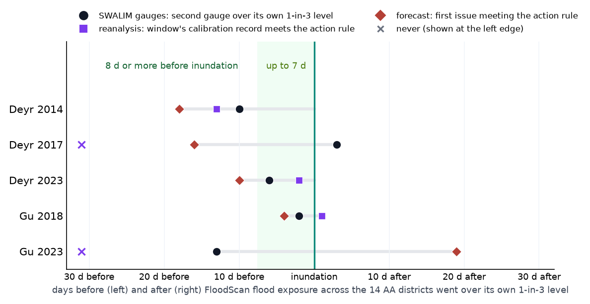
The forecasts came eight days or more before the inundation in 3 of the 5 seasons (Deyr 2014 (+18 d), Deyr 2017 (+16 d), Deyr 2023 (+10 d)), all Deyr on GloFAS v4; on the day or up to seven days before in 1 (Gu 2018 (+4 d)); and after it in 1 (Gu 2023 (-19 d)), the season every source missed. The SWALIM gauges, the benchmark the rest of this page is scored against, sit 2 to 13 days before the inundation and three days after it in Deyr 2017, a season the gauges called on the Juba while the exposure came on the Shabelle. The reanalysis, the record the windows were calibrated on, never met the rule in Deyr 2017 or Gu 2023 and met it a day after the crossing in Gu 2018.
| season | exposure crossed 1-in-3 | SWALIM gauges, 2nd over 1-in-3 | reanalysis rule met | first forecast issue | |||
|---|---|---|---|---|---|---|---|
| date | lead | date | lead | date | lead | ||
| Deyr 2006 | below 1-in-3 | 2006-10-30 | – | 2006-10-29 | – | never | – |
| Deyr 2008 | below 1-in-3 | 2008-11-15 | – | never | – | never | – |
| Deyr 2014 | 2014-10-30 | 2014-10-20 | +10 d | 2014-10-17 | +13 d | 2014-10-12 | +18 d |
| Deyr 2017 | 2017-11-04 | 2017-11-07 | -3 d | never | – | 2017-10-19 | +16 d |
| Deyr 2019 | below 1-in-3 | 2019-10-14 | – | 2019-10-13 | – | 2019-10-02 | – |
| Deyr 2020 | below 1-in-3 | 2020-10-01 | – | never | – | 2020-10-02 | – |
| Deyr 2023 | 2023-10-31 | 2023-10-25 | +6 d | 2023-10-29 | +2 d | 2023-10-21 | +10 d |
| Gu 2016 | below 1-in-3 | 2016-05-01 | – | 2016-05-07 | – | 2016-04-30 | – |
| Gu 2018 | 2018-04-19 | 2018-04-17 | +2 d | 2018-04-20 | -1 d | 2018-04-15 | +4 d |
| Gu 2020 | below 1-in-3 | 2020-04-22 | – | 2020-04-29 | – | 2020-04-22 | – |
| Gu 2023 | 2023-04-07 | 2023-03-25 | +13 d | never | – | 2023-04-26 | -19 d |
The comparison is thin: eleven benchmark seasons have a forecast archive and five of them an inundation day. The exposure record calls seasons the gauges do not, mostly on the Shabelle, and stays below its level in several gauge floods. At 10 km FloodScan blurs the river with rain on the floodplain, and exposure follows population, so the lower Shabelle weighs heavily in it. The flood-benchmark step kept the gauges as the benchmark for those reasons. What the comparison adds is a direction: where the benchmark errs on timing it errs late, on the Shabelle, and the reach it misses is the one below the last gauge.
Calibrated on the reanalysis, checked on the forecasts
Refitting the same rule on the forecast archives themselves, 2003–2023, thresholds from 1-in-3 to 1-in-5. Out of the field: Google GRRR, whose archive is too short to carry a 1-in-3 threshold, so it can only be calibrated on the retrospective.
| window | source | gauge threshold | points that must agree | would have activated in |
|---|---|---|---|---|
| Juba Gu | GloFAS v4 | 1-in-3 | 2 of 4 | 2005, 2010, 2013, 2016, 2018, 2020, 2023 |
| Juba Deyr | GloFAS v4 | 1-in-5 | 3 of 4 | 2015, 2017, 2023 |
| Shabelle Gu | GloFAS v4 | 1-in-4 | 2 of 3 | 2005, 2010, 2016, 2018 |
| Shabelle Deyr | GloFAS v4 | 1-in-5 | 2 of 3 | 2010, 2013, 2019, 2020 |
Envelope 1-in-2.2 (10 of 21 years), catching 5 of the 7 severe years (2006 and 2014 missed). This is the closest rate the forecast record supports; nothing lands on 1-in-3.
Supporting evidence: the tuning surface
The tuning surface
The Nigeria-style grid search (per state there; per river and season here, the same recipe as P. Wairimu's notebook 08): every (station return period, gauges required) cell is scored against the seasonal SWALIM benchmark for the window's adopted model. The adopted cell is not always the best single-window score: it is the cell the envelope search picked under this page's constraints (thresholds 1-in-3 to 1-in-6, at least two gauges but never all of them, the union of the four windows at 1-in-3 or rarer with the most severe years caught). The neighbours show what loosening a window would cost in false activations, or tightening one in missed severe years.

Supporting evidence: official SWALIM levels vs the fitted ones
How the official SWALIM levels compare with the fitted ones
The benchmark years above are defined by empirical return periods of the
gauges' own seasonal maxima, not by SWALIM's published Moderate/High
flood-risk levels. The check below is why. Putting the official levels on the
empirical RP scale (per active gauge and season, 1999–2023) shows they imply wildly
inconsistent frequencies: "Moderate" ranges from a level the river reaches most
years (Dollow Deyr, ~1-in-1.3; Jowhar Gu, ~1-in-1.6) to a genuinely rare one (Luuq
Gu, ~1-in-4.6), and "High" from ~1-in-1.8 (Dollow) to ~1-in-11.5 (Luuq Gu). They
are engineering levels of uncertain provenance rather than a consistent severity scale, the same conclusion P. Wairimu's notebook 01 flagged when the published
max_level at Belet Weyne came out below its bank-full level.
Everything in this mechanism therefore runs on each gauge's own empirical RP3/RP5
levels (table som_ms_swalim_rp); the official levels remain useful
only as familiar reference lines for readers of SWALIM bulletins.

Would it have worked operationally?
The calibration record is reanalysis, a model's afterwards-view of its own past. The operational test replays the historical forecasts. A forecast has two dates: the issue date, when it was published, and the valid day, the day it describes. Per point and valid day, the most alarming signal at leads 1 to 7 (max over issue dates). Google windows use their own reforecast (2016–2023); GloFAS v5 windows the v4 reforecast (2003–2023, ensemble median, thresholds refit on v4's own climatology, since no v5 reforecast exists); GEOGloWS windows the retrospective as a lead-0 stand-in (hindsight, flagged per window). That forecast skill barely decays from lead 1 to 7 on these slow rivers, where the flow is driven by initial conditions, is P. Wairimu's notebook 03 finding, and is what makes both lead bands viable at all.
| window | calibrated on | run on | reproduces its calibration years? |
|---|---|---|---|
| Juba Gu | Google GRRR reanalysis | Google GRRR forecasts, leads 1-7 | yes, same archive |
| Juba Deyr | GloFAS v5 reanalysis | GloFAS v4 operationally, levels refit on v4's climatology, until a v5 forecast exists; lead-time evidence from GloFAS v4 | cannot be shown directly: no reforecast for this version |
| Shabelle Gu | Google GRRR reanalysis | Google GRRR forecasts, leads 1-7 | yes, same archive |
| Shabelle Deyr | GloFAS v5 reanalysis | GloFAS v4 operationally, levels refit on v4's climatology, until a v5 forecast exists; lead-time evidence from GloFAS v4 | cannot be shown directly: no reforecast for this version |
The readiness leg (8–12 days)
Readiness covers leads 8 to 12 days, the days beyond the action window, and runs on GloFAS v4 ensemble-median forecasts over the same full set of points, against the same reanalysis levels as the action leg, at the window's return period capped at 1-in-5 (the 21-year reforecast archive does not resolve rarer levels). One issue at a time: the points must be over their levels on the same issue and the same valid day. The reforecast archive at these leads runs 2003 to 2023. Readiness releases only the mobilisation share and is held to the same floor: no threshold below 1-in-3.
| window | readiness rule | readiness years | covers action years |
|---|---|---|---|
| Juba Gu | 3 of 4 points over 1-in-5 | 2020 | 1 of 4 |
| Juba Deyr | 3 of 4 points over 1-in-4 | 2017, 2023 | 1 of 2 |
| Shabelle Gu | 2 of 3 points over 1-in-5 | 2005, 2010, 2016 | 1 of 4 |
| Shabelle Deyr | 2 of 3 points over 1-in-5 | 2013, 2019 | 1 of 4 |
Readiness carries each window's own rule, the same votes and the same return period capped at 1-in-5, against the same reanalysis levels as the action leg. Across the four windows it is reached in 8 of the 21 archive years (1-in-2.8): 2005, 2010, 2013, 2016, 2017, 2019, 2020 and 2023.
Resolved 2026-09-07 for the overlap: readiness is stated as 8 to 12 days everywhere on the page. Since 2026-09-18 the readiness leg reads the reanalysis levels, so the 8-to-12-day forecast archive no longer enters the thresholds. Original note: action runs at leads 1–7 and readiness at leads 7–12, both inclusive, so lead 7 sits in both bands and the same forecast day can serve either leg. The original specification was action under 6 days. Separately, the “covers action years” column is a season-year set intersection: it records that both legs activated in the same season, not that readiness came first.
Counting across the four windows on the reanalysis levels: Juba Gu 1 of 4 covered, Juba Deyr 1 of 2, Shabelle Gu 1 of 4, Shabelle Deyr 1 of 4. The uncovered activations include Shabelle Deyr 2023, the largest flood in the record, and Shabelle Gu 2018 and 2020. Under the staged model that would have been a design failure; under the 2026-08-27 decision it is accepted, but the working group should see the count before accepting it.
Return-period bookkeeping
| level | trigger | activations (1999-2023) | RP |
|---|---|---|---|
| individual | Juba Gu action | 4: 2013, 2016, 2018, 2020 | 6.5 yr |
| individual | Juba Deyr action | 2: 2006, 2023 | 13.0 yr |
| individual | Shabelle Gu action | 4: 2013, 2016, 2018, 2020 | 6.5 yr |
| individual | Shabelle Deyr action | 4: 2006, 2014, 2019, 2023 | 6.5 yr |
| river | Juba (Gu or Deyr) | 6 | 4.3 yr |
| river | Shabelle (Gu or Deyr) | 8 | 3.2 yr |
| overall | action, either river | 8 | 3.2 yr |
Under all-in funding, where any activation releases the full envelope, the effective return period is the overall row: 1-in-3.2 with Google, 1-in-3.2 without. The individual windows are set rarer than that on purpose, because four windows each calibrated to 1-in-3 give a union of roughly 1-in-1.5.
Activations, impact and response, year by year
The two-historical-records rule: the trigger record against impact, not just the hazard benchmark. Everything is grouped river → season, reverse-chronological. The trigger column is the trigger's actual decision variable: the peak number of monitored points simultaneously over their thresholds that season-year. The cell fills red when it meets the requirement shown in the season header (= the trigger activates). RP is the two-gauge benchmark used throughout this page: 5yr when at least two of the river's gauges reached their own 1-in-5 level that season, 3yr when two reached 1-in-3 but not 1-in-5 (Weibull on each gauge's own seasonal maxima from 2000, not the official flood-risk levels); EM-DAT (purple) is people affected and CERF (blue) the allocation from the UN Central Emergency Response Fund (US$), shaded by magnitude, each attributed to the river(s) named in the event or allocation narrative.
| loading… |
Attribution & caveats. EM-DAT is a floor (entry-criteria bias), split to seasons by start month (Mar–Jun → Gu, Sep–Dec → Deyr); an event naming both rivers is counted under both rivers (not split; hover for deaths and the multi-river flag); events naming neither river (mostly flash floods elsewhere) are excluded. A CERF allocation naming neither river in its narrative is shown under both rivers and marked * (they are national riverine-flood responses). Impact columns are context, not a skill score: a formal skill-vs-impact statistic still requires choosing an impact threshold.
Gu 2024, the one year outside this record, was severe at the Shabelle gauges (all three over their 1-in-5) and a 1-in-3 flood at the Juba gauges (Luuq at its 1-in-5, Dollow just under). It cannot be replayed on Google, whose archive ends in 2023. Replayed on the operational GloFAS v4 forecasts, the Juba window activates on the action leg on 6 May, two days before Luuq's peak, with all four points over their levels by 7 May; the Shabelle window does not activate on either leg, its forecast peaks in early May reaching only 75–86% of the action levels, consistent with the v4 blind spot behind the missed Deyr 2023.
SWALIM's alerts against the trigger
SWALIM, the Somalia Water and Land Information Management project run by FAO, issues its own flood bulletins from the gauge readings and the rainfall forecast, grading river flood risk as moderate, then high, then bank full or overflow. The question here is who flagged first in each flood season, SWALIM or the trigger, and by how many days. Every date is the date the information was available: the issue date of the SWALIM bulletin, the first day the trigger crossed on its reanalysis (Google for Gu, GloFAS v5 for Deyr), and, in Deyr only, the issue date of the first GloFAS v4 forecast (the live stand-in for GloFAS v5, which has no forecast) whose ensemble median had enough points over their thresholds at some lead of 1 to 7 days. v4 is not the Gu model and is not shown on Gu rows. The grey band marks the gauges' own two-gauge 1-in-3 and 1-in-5 crossings.

The action window is 1 to 7 days before the flood and readiness 8 to 12. The chart below places each flag against the onset of the flood at the gauges, the day the two-gauge 1-in-3 level was first crossed, not the peak. The trigger's date is the day the modelled flow crossed; in operation the forecast would have added up to 7 days to it. The GloFAS v4 issue date is the operational measure.

SWALIM's first bulletin fell inside the action window in five of the twelve seasons with a bulletin and a gauge event: Deyr 2006 and Deyr 2014 on the Shabelle, Deyr 2014 and Deyr 2023 on the Juba, and Gu 2024 on the Juba, at 1 to 7 days before onset. It was earlier than the action window in three (Gu 2020 Shabelle 8 days, inside the readiness window; Deyr 2023 Shabelle 16 days; Gu 2024 Shabelle 19 days) and on or after onset in four (Deyr 2006 Juba, Deyr 2019 Shabelle, Gu 2020 Juba, Gu 2023 Shabelle). In Deyr, the GloFAS v4 issue was in the action window in 2023 on the Juba (4 days before onset), in the readiness window in 2014 and 2019 on the Shabelle (8 and 12 days), and on or after onset or absent in the other seasons. The reanalysis trigger's own day was inside the action window in Deyr 2006 on the Juba and in Deyr 2014, Deyr 2019 and Gu 2020 on the Shabelle; it was on or after onset in five seasons (Deyr 2006 and Deyr 2023 on the Shabelle, Deyr 2023 and Gu 2020 on the Juba, Gu 2016 on the Shabelle), which is the gap a 1 to 7 day forecast has to close; and it was never reached in Deyr 2014 on the Juba and in Deyr 2020 and Gu 2023 on the Shabelle.
Where both flagged, SWALIM was first in six river-seasons and the window's model in two. SWALIM's lead was 2 to 3 days in Deyr 2006, Deyr 2014 and Gu 2020, and 9 and 20 days in Deyr 2023, when its 20 October alert asked for anticipatory action and GloFAS v5 crossed on 29 October on the Juba and 10 November on the Shabelle. GloFAS v5 led in Deyr 2019 on the Shabelle by 9 days and in Deyr 2006 on the Juba by 2 days, where SWALIM's earlier issues are missing. In four flood seasons SWALIM flagged and the model never crossed: GloFAS v5 in Deyr 2014 and Deyr 2019 on the Juba, Google in Gu 2021 on both rivers and Gu 2023 on the Shabelle. In Deyr 2020 on the Shabelle the model did not cross either, and SWALIM's only bulletin concerned the September flood. Gu 2016 has no SWALIM bulletin at all.
The GloFAS v4 forecast, which is what would run live, is earlier than SWALIM where it crosses at all in Deyr: by 3 days in Deyr 2014 and 20 days in Deyr 2019 on the Shabelle, with SWALIM ahead in Deyr 2014 on the Juba (8 days) and Deyr 2023 on the Juba (1 day). On the Juba in Gu, where v4 is not the window's model, the same replay was 4 days behind SWALIM in 2020 and 4 days ahead in 2024. No v4 issue had a point over its level in Gu 2020, Deyr 2023 or Gu 2024 on the Shabelle, three seasons in which SWALIM reported bank full at Belet Weyne. Most of SWALIM's archived bulletins up to 2021 are Flood Updates written once a river was already at the high level or bank full; a moderate-risk step is recorded in Deyr 2014, Gu 2020 on the Shabelle, Gu 2021 and from 2023.
The same comparison station by station
The charts above work at river level, where SWALIM's earliest flag anywhere on the river meets a rule that counts points. SWALIM's bulletins name individual gauges and publish their readings, so the same comparison can be made gauge by gauge. The two charts below give one row per station and season: the bulletin on which SWALIM first reported that gauge at each of its own official levels, that gauge's own return-period crossings, and the first day each model crossed that station's own threshold. A level counts as reported when the reading SWALIM published for the gauge is at or above its official moderate, high or bank-full level. Hollow markers are seasons where the bulletin stated a risk for the station without publishing a reading, which is most of 2006 and 2019 to 2021. The 2024 weekly bulletins are read from their published readings only, because their prose mixes forecasts and look-backs to earlier years.


Of the 55 station-seasons, 39 have a bulletin naming that gauge and 21 record it at bank full. Belet Weyne and Jowhar are named in 8 of their 9 seasons, Bulo Burti in 6; on the Juba, Luuq in 6 of 7, Dollow and Bardheere in 4, Bualle in 3. Where the gauge crossed its own 1-in-3 and no bulletin named the station, the gap falls on Bulo Burti and Bardheere twice each and on Belet Weyne and Bualle once.
The station view separates two things the river view combines. SWALIM is early at Belet Weyne, flagging it before or on the day the gauge crossed its own 1-in-3 in seven of eight seasons and 8 days late in the eighth. It is late at Luuq in all five seasons with both dates, by 1 to 16 days, and at Bulo Burti in four of six. Jowhar is the exception to the whole comparison: in three of its eight flagged seasons the gauge never crossed its own 1-in-3, which matches the bulletins describing flooding there from breakages at Baarey, Moyko and Mandheere rather than from the river topping its banks.
Against SWALIM's first flag for the same gauge, over the 34 station-seasons up to 2023, Google crossed that station's threshold earlier in 15, on the same day in 2, later in 8 and never in 9. GloFAS v5 was earlier in 12, on the same day in 1, later in 12 and never in 9. The GloFAS v4 forecast issue was earlier in 7, same day in 3, later in 7 and absent in 17. At station level the models therefore lead SWALIM about as often as they trail it, and the trigger's advantage at river level comes from requiring several points rather than from any one gauge being called early.
Full record: the bulletins, the points over and the peaks
For each river-season the table gives what happened at the gauges, the bulletin that first reported each step of SWALIM's ladder (with the station and level the bulletin gives; where the bulletin dates the crossing to an earlier day, that day follows the level), the trigger's first day with the points over their return-period thresholds, the GloFAS v4 forecast's first issue with enough points over and the valid day it pointed at ("issued 20 Oct for 21 Oct"), and the same rule on the GloFAS v5 reanalysis for every window. Each model cell then gives the season's peak count and how many days (or forecast issues) stayed at or above the required count; where the rule never crossed, the most points over on any one day. The lag columns count days from SWALIM's first bulletin flagging any level (positive when SWALIM was earlier).
Sources: the 52 bulletins in the SWALIM archive on blob (raw/swalim/alerts/),
which carry river bulletins for 2016 and 2019 to 2023; SWALIM's Flood Watch, Flood
Alert and Flood Update bulletins for Deyr 2006 and Deyr 2014 retrieved from ReliefWeb;
and for Gu 2024 the river-level section of SWALIM's weekly weather bulletins, since no
separate flood alert was issued that season. The 2008 and 2018 flood seasons have no
bulletins yet. The v4 forecast column uses the twice-weekly 11-member reforecast up to
2023 and, for Gu 2024, the daily 50-member operational forecasts archived for that
season.
| season | river | what happened at the gauges | SWALIM: moderate risk | SWALIM: high risk | SWALIM: bank full or overflow | trigger: first day and points over their RP | days SWALIM's first bulletin led the trigger | GloFAS v4 forecast, by issue date (Deyr only) | days SWALIM's first bulletin led the v4 issue | GloFAS v5 reanalysis |
|---|---|---|---|---|---|---|---|---|---|---|
| Deyr 2006 | Juba | Severe flood; 1-in-3 and 1-in-5 on 30 Oct | not archived (bulletin no. 1 of 3 Oct saw no risk; nos. 2 to 7 missing) | 31 Oct, high risk in the riverine areas | 31 Oct, river over its banks from Luuq to Jamame | 29 Oct, 3 of 4: Luuq, Bardheere, Bualle peak 3 of 4 that day; 5 days at or above the count | -2 | no no point over its level in any issue | 29 Oct, 3 of 4: Luuq, Bardheere, Bualle peak 3 of 4 that day; 5 days at or above the count | |
| Deyr 2006 | Shabelle | Severe flood; 1-in-3 on 2 Nov, 1-in-5 on 11 Nov | not archived (nos. 2 to 7 missing) | 31 Oct, severe risk downstream of Jowhar | 31 Oct, bank breakages in the lower Shabelle after abrupt rises at Belet Weyne, Bulo Burti and Jowhar | 2 Nov, 2 of 3: Belet Weyne, Bulo Burti peak 3 of 3 on 4 Nov: Belet Weyne, Bulo Burti, Jowhar; 10 days at or above the count | +2 | no most: 1 of 3, issued 30 Oct for 30 Oct: Jowhar | 2 Nov, 2 of 3: Belet Weyne, Bulo Burti peak 3 of 3 on 4 Nov: Belet Weyne, Bulo Burti, Jowhar; 10 days at or above the count | |
| Deyr 2014 | Juba | Severe flood; 1-in-3 on 22 Oct, 1-in-5 on 24 Oct | 15 Oct, both rivers | 21 Oct, both rivers | 28 Oct, floods at Dollow, Jilib and Jamame (24 Oct: Luuq 1 m below bank full) | no no point over its level | issued 23 Oct for 25 Oct, 3 of 4: Dollow, Luuq, Bardheere peak 4 of 4 issued 24 Oct for 25 Oct: Dollow, Luuq, Bardheere, Bualle; 4 issues at or above the count | +8 | no no point over its level | |
| Deyr 2014 | Shabelle | Severe flood; 1-in-3 on 20 Oct, 1-in-5 on 29 Oct | 15 Oct, Belet Weyne 6.10 m | 20 Oct, Flood Alert: Belet Weyne 7.00 m past the critical level | 24 Oct, Belet Weyne 7.30 m, the flooding level; 28 Oct floods at Belet Weyne and breakages in Middle Shabelle | 17 Oct, 2 of 3: Belet Weyne, Bulo Burti peak 3 of 3 on 19 Oct: Belet Weyne, Bulo Burti, Jowhar; 7 days at or above the count | +2 | issued 12 Oct for 13 Oct, 2 of 3: Belet Weyne, Bulo Burti peak 2 of 3 in that issue; 1 issue at or above the count | -3 | 17 Oct, 2 of 3: Belet Weyne, Bulo Burti peak 3 of 3 on 19 Oct: Belet Weyne, Bulo Burti, Jowhar; 7 days at or above the count |
| Gu 2016 | Shabelle | Severe flood; 1-in-3 on 11 May, 1-in-5 on 18 May | no bulletin archived | no bulletin archived | no bulletin archived (June flood map only) | 12 May, 3 of 3: Belet Weyne, Bulo Burti, Jowhar peak 3 of 3 that day; 4 days at or above the count | not the Gu model | 15 May, 2 of 3: Belet Weyne, Bulo Burti peak 3 of 3 on 17 May: Belet Weyne, Bulo Burti, Jowhar; 11 days at or above the count | ||
| Deyr 2019 | Juba | No two-gauge crossing; local flooding reported | not archived; the 25 Oct update says the moderate level was passed in the two weeks before 22 Oct | 22 Oct, Bardheere | 22 Oct, Bardheere bank full, flooding at Luuq and Bardheere; 25 Oct also Dollow and Bualle | no most: 2 of 4 on 15 Oct: Luuq, Bardheere | no no point over its level in any issue | no most: 2 of 4 on 15 Oct: Luuq, Bardheere | ||
| Deyr 2019 | Shabelle | Severe flood; 1-in-3 on 14 Oct, 1-in-5 on 22 Oct | not archived (first bulletin 22 Oct) | 22 Oct, Belet Weyne and Jowhar (Jowhar at the high level since late August) | 22 Oct, Jowhar near bank full with two breakages; 25 Oct Belet Weyne town flooded by overflow | 13 Oct, 2 of 3: Belet Weyne, Bulo Burti peak 3 of 3 on 15 Oct: Belet Weyne, Bulo Burti, Jowhar; 22 days at or above the count | -9 | issued 2 Oct for 2 Oct, 3 of 3: Belet Weyne, Bulo Burti, Jowhar peak 3 of 3 in that issue; 9 issues at or above the count | -20 | 13 Oct, 2 of 3: Belet Weyne, Bulo Burti peak 3 of 3 on 15 Oct: Belet Weyne, Bulo Burti, Jowhar; 22 days at or above the count |
| Deyr 2020 | Shabelle | 1-in-3 on 1 Oct, 1-in-5 on 6 Oct (a separate flood at Belet Weyne in September) | no bulletin for the October rise | 8 Sep, Bulo Burti 7.00 m (the September flood) | 8 Sep, Belet Weyne bank full with overbank spillage | no no point over its level | issued 2 Oct for 3 Oct, 3 of 3: Belet Weyne, Bulo Burti, Jowhar peak 3 of 3 in that issue; 4 issues at or above the count | no no point over its level | ||
| Gu 2020 | Juba | Severe flood; 1-in-3 on 22 Apr, 1-in-5 on 12 May | not archived (first bulletin 27 Apr) | 27 Apr, Bardheere passed the high level that morning | 27 Apr, flooding reported at Dollow, Luuq and Bardheere | 29 Apr, 3 of 4: Dollow, Bardheere, Bualle peak 4 of 4 on 30 Apr: Dollow, Luuq, Bardheere, Bualle; 20 days at or above the count | +2 | not the Gu model | 30 Apr, 3 of 4: Luuq, Bardheere, Bualle peak 4 of 4 on 11 May: Dollow, Luuq, Bardheere, Bualle; 11 days at or above the count | |
| Gu 2020 | Shabelle | Severe flood; 1-in-3 on 5 May, 1-in-5 on 12 May | 27 Apr, high risk foreseen with Belet Weyne still 0.50 m below the moderate level; 4 May, Belet Weyne 7.20 m past it | 4 May, Jowhar at the high level for four days; 11 May, Belet Weyne 8.10 m over it | 18 May, Belet Weyne bank full since 12 May; 11 May Jowhar 0.20 m below | 30 Apr, 3 of 3: Belet Weyne, Bulo Burti, Jowhar peak 3 of 3 that day; 16 days at or above the count | +3 | not the Gu model | 3 May, 2 of 3: Belet Weyne, Bulo Burti peak 3 of 3 on 5 May: Belet Weyne, Bulo Burti, Jowhar; 19 days at or above the count | |
| Gu 2021 | Juba | No two-gauge crossing | 10 May, Dollow over the moderate level, Luuq 0.30 m below | not reached (high risk foreseen on 10 May; risk down to minimal on 19 May) | no | no no point over its level | not the Gu model | no no point over its level | ||
| Gu 2021 | Shabelle | Belet Weyne flooded; gauge censored at bank full, no two-gauge crossing | 10 May, Belet Weyne 6.50 m | 19 May, Belet Weyne 7.60 m (13 May: 6.60 m with high risk stated) | 25 May, Belet Weyne 8.25 m about to reach bank full; 19 May breakage flooding upstream reported | no no point over its level | not the Gu model | no no point over its level | ||
| Gu 2023 | Shabelle | Severe flood; 1-in-3 on 17 Apr, 1-in-5 on 18 May | no bulletin archived | 8 May advisory: high level at Belet Weyne, passed on 2 May | 8 May advisory: 0.40 m below bank full, overflow judged very likely | no no point over its level | not the Gu model | no no point over its level | ||
| Deyr 2023 | Juba | Severe flood; 1-in-3 and 1-in-5 on 25 Oct | 20 Oct, Dollow and Luuq (Flood Alert with a call for anticipatory action) | 23 Oct update: high level passed at Luuq on 21 Oct and Bardheere on 22 Oct; 29 Oct all three over it | 13 Nov advisory: overflow along the whole river for more than a week | 29 Oct, 3 of 4: Dollow, Luuq, Bardheere peak 4 of 4 on 30 Oct: Dollow, Luuq, Bardheere, Bualle; 37 days at or above the count | +9 | issued 21 Oct for 21 Oct, 4 of 4: Dollow, Luuq, Bardheere, Bualle peak 4 of 4 in that issue; 11 issues at or above the count | +1 | 29 Oct, 3 of 4: Dollow, Luuq, Bardheere peak 4 of 4 on 30 Oct: Dollow, Luuq, Bardheere, Bualle; 37 days at or above the count |
| Deyr 2023 | Shabelle | Largest flood on record; 1-in-3 on 6 Nov, 1-in-5 on 19 Nov | 29 Oct, moderate risk along the river with Belet Weyne 0.10 m below the level (21 Oct advisory: anticipatory action called for Hiraan) | 2 Nov, high risk projected at Belet Weyne in 3 to 4 days | 13 Nov advisory: Belet Weyne overflowing, most of the town flooded; 20 Nov Bulo Burti 0.32 m over the high level | 10 Nov, 2 of 3: Belet Weyne, Bulo Burti peak 3 of 3 on 11 Nov: Belet Weyne, Bulo Burti, Jowhar; 22 days at or above the count | +20 | no no point over its level in any issue | 10 Nov, 2 of 3: Belet Weyne, Bulo Burti peak 3 of 3 on 11 Nov: Belet Weyne, Bulo Burti, Jowhar; 22 days at or above the count | |
| Gu 2024 | Juba | 1-in-3 flood on 10 May (Luuq 7 May, Dollow 10 May); no gauge reached 1-in-5 (Luuq peaked 0.02 m below its level on 8 May) | 9 May weekly bulletin: Luuq over the moderate level (8 May reading) | 9 May weekly bulletin: Dollow over the high level on 6 May after very heavy rain, back below it by 9 May | no (14 May: Dollow below the flood levels) | not available: record ends 2023 | not the Gu model | not available: record ends 2023 | ||
| Gu 2024 | Shabelle | Severe flood; 1-in-3 on 8 May (Jowhar 19 Apr, Belet Weyne 8 May), 1-in-5 on 20 May | 1 May weekly bulletin: Belet Weyne 6.50 m | 19 Apr weekly bulletin: Jowhar 0.23 m below bank full; 9 May: Belet Weyne 7.48 m | 22 May weekly bulletin: Belet Weyne 8.30 m bank full with riverine flooding reported; 14 May: breakage floods at three villages on 12 May | not available: record ends 2023 | not the Gu model | not available: record ends 2023 | ||
SWALIM's bulletins in seasons the gauges did not call a flood
The 24 seasons between 2006 and 2023 in which neither river crossed the two-gauge 1-in-3 are the test of whether SWALIM raises risk for rises that come to nothing. ReliefWeb holds SWALIM bulletins for 15 of them. For each, the table shows the highest level SWALIM reached, what it reported, and what the impact and trigger records hold for the same season.
All 24 seasons: what SWALIM issued and what was reported
| season | bulletins | highest level SWALIM reached | when | what SWALIM reported | other records |
|---|---|---|---|---|---|
| Gu 2006 | 0 | no bulletins found | |||
| Gu 2007 | 6 | moderate risk | 24 Apr-30 May | 30 May: bank breakage at Marerey (Jowhar) closed, Madera breakage still open | |
| Deyr 2007 | 10 | high risk or alert | 23 Oct (lower Juba) | OCHA sitreps: three bank breakages at Belet Weyne (28 Sep), Shabelle at 5.2 m with overflow expected at 5.25 m that did not occur (5 Oct); no villages inundated (12 Oct) | EM-DAT 8,000 affected (Shabelle) |
| Gu 2008 | 0 | no bulletins found | |||
| Gu 2009 | 8 | none above minimal | eight weekly watches, no risk statement above minimal | ||
| Deyr 2009 | 10 | moderate risk | 27 Oct; 3 Nov | moderate risk lower Shabelle (27 Oct) then lower reaches of both rivers (3 Nov); none in the other 8 watches | EM-DAT 1,750 affected |
| Deyr 2010 | 2 | high risk or alert | 28 Sep; 3 Nov | 28 Sep: river 76 cm above the high-risk flood level; 3 Nov: 3.5 cm above the high-risk level | |
| Gu 2011 | 0 | no bulletins found | |||
| Deyr 2011 | 12 | moderate risk | 17 Oct-1 Nov; 6 Dec | 5 Dec flash flood update: Luuq 5.90 m, 40 cm above the critical level of flooding | |
| Gu 2012 | 4 | none above minimal | watches 8 May-5 Jun: minimal or no risk | ||
| Deyr 2012 | 5 | moderate risk | 23 Oct-13 Nov | 28 Sep Flood Alert: 188 mm rain at Belet Weyne, river at bank full 8.30 m (flash flood, before the Deyr window) | EM-DAT 32,200 affected |
| Gu 2013 | 8 | high risk or alert | 10 Apr-6 May | OCHA flood infographic 30 Apr: flooding reported in the south; 20 May watch: breakages in the lower Shabelle not yet closed | EM-DAT 50,000 affected; adopted trigger activated on both rivers |
| Deyr 2013 | 8 | high risk or alert | 29 Oct-27 Nov | 7 Nov Flood Alert: river breakages at Luuq, farmland inundated | adopted trigger did not activate |
| Gu 2014 | 5 | none above minimal | four watches 6 May-3 Jun, no risk statement above minimal | ||
| Gu 2015 | 10 | high risk or alert | 28 Apr-12 May | high risk middle and lower Shabelle for three weekly watches; back to moderate 20 May and minimal 2 Jun; benchmark and adopted trigger: nothing | EM-DAT 16,296 affected (Shabelle) |
| Deyr 2015 | 12 | high risk or alert | 6 Nov-13 Nov (OCHA flash updates quoting SWALIM); Shabelle River Flood Alert 23 Oct | floods reported in Jamame and Jilib in October; Bulo Burti over its moderate-risk level 4 Nov (5.38 m vs 5.00); breakages at Balcad, Jowhar, Mahaday | |
| Deyr 2016 | 0 | no bulletins found | |||
| Gu 2017 | 3 | high risk or alert | 10-17 May | river levels rose significantly on both rivers after the rains, high risk stated in two watches; no benchmark crossing, no activation, no | |
| Deyr 2018 | 0 | no bulletins found | adopted record had 2 Juba points over (3 needed) | adopted record: 2 Juba points over, 3 needed | |
| Gu 2019 | 0 | no bulletins found | |||
| Gu 2021 | 5 | high risk or alert | 19-25 May | 19 May: flooding reported upstream of Belet Weyne (Bacaad, Qooqane, Laffole, Grash, Nimcan, Leboow, Shinile); 25 May: Belet Weyne 8.25 m, about to reach bank full | EM-DAT 400,000 affected |
| Deyr 2021 | 0 | no bulletins found | |||
| Gu 2022 | 0 | no bulletins found | |||
| Deyr 2022 | 0 | no bulletins found |
SWALIM stayed at minimal risk in 3 of the 15 seasons, went to moderate in 4, and to high risk or an alert in 8. In six of the eight there is flooding on record elsewhere. EM-DAT counts people affected in Gu 2013 (50,000), Gu 2015 (16,000), Gu 2021 (400,000) and Deyr 2007 (8,000); breakages and reported floods appear in the Deyr 2013 and Deyr 2015 bulletins. Deyr 2010 and Gu 2017 are the two seasons with a high flag and nothing else on record. These floods sat below the two-gauge 1-in-3 the trigger is built on, at one gauge or along one stretch of river. The moderate flag appears in most rainy seasons with any rise; SWALIM uses it as a watch. In Gu 2013, when the adopted trigger activated without the gauge benchmark, SWALIM held high risk for four weeks; in Deyr 2013, when it did not activate, for five weeks.
SWALIM also reported two floods that neither the gauge benchmark nor any model registered: Gu 2021 at Belet Weyne, where the gauge reading stopped at bank full, and Gu 2023 at Belet Weyne. Risk levels in the table are read from the bulletin text by keyword and were spot-checked, not read in full; first-flag dates are the earliest bulletins found, not necessarily SWALIM's first communication.
When each model would have flagged, year by year
One timeline per window, one row per year from 1999 to 2023, on calendar dates within the season. Each model runs the window's point count over 1-in-3 station levels fitted on its own reanalysis, rather than the adopted 1-in-4 to 1-in-6, so this is the earliest a flag could reasonably have come; the years without a gauge flood show what that costs in extra flags. Diamonds are the first day the reanalysis crossed (Google in blue, GloFAS v5 in teal). Triangles are the first forecast issue that crossed at leads 1 to 7: the Google reforecast covers 2016 to mid-2023, the GloFAS v4 reforecast 2003 to 2023 at two issues a week. The grey band runs from the gauges' two-gauge 1-in-3 crossing to their 1-in-5 crossing, and an asterisk marks a severe year. The text at right gives days before or after the gauges' 1-in-3 crossing, or, in years without a gauge flood, which models flagged. The Juba gauges did not report in 1999 to 2001 and the Shabelle gauges in 1999.
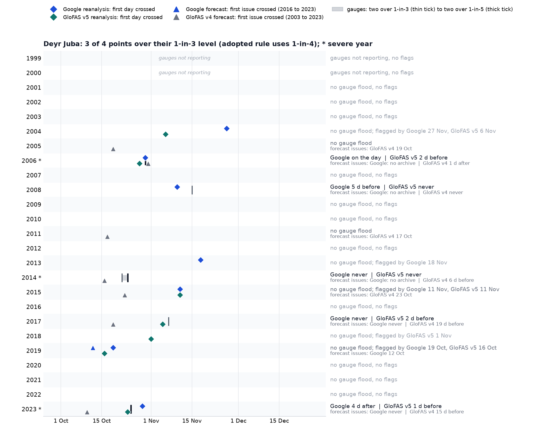
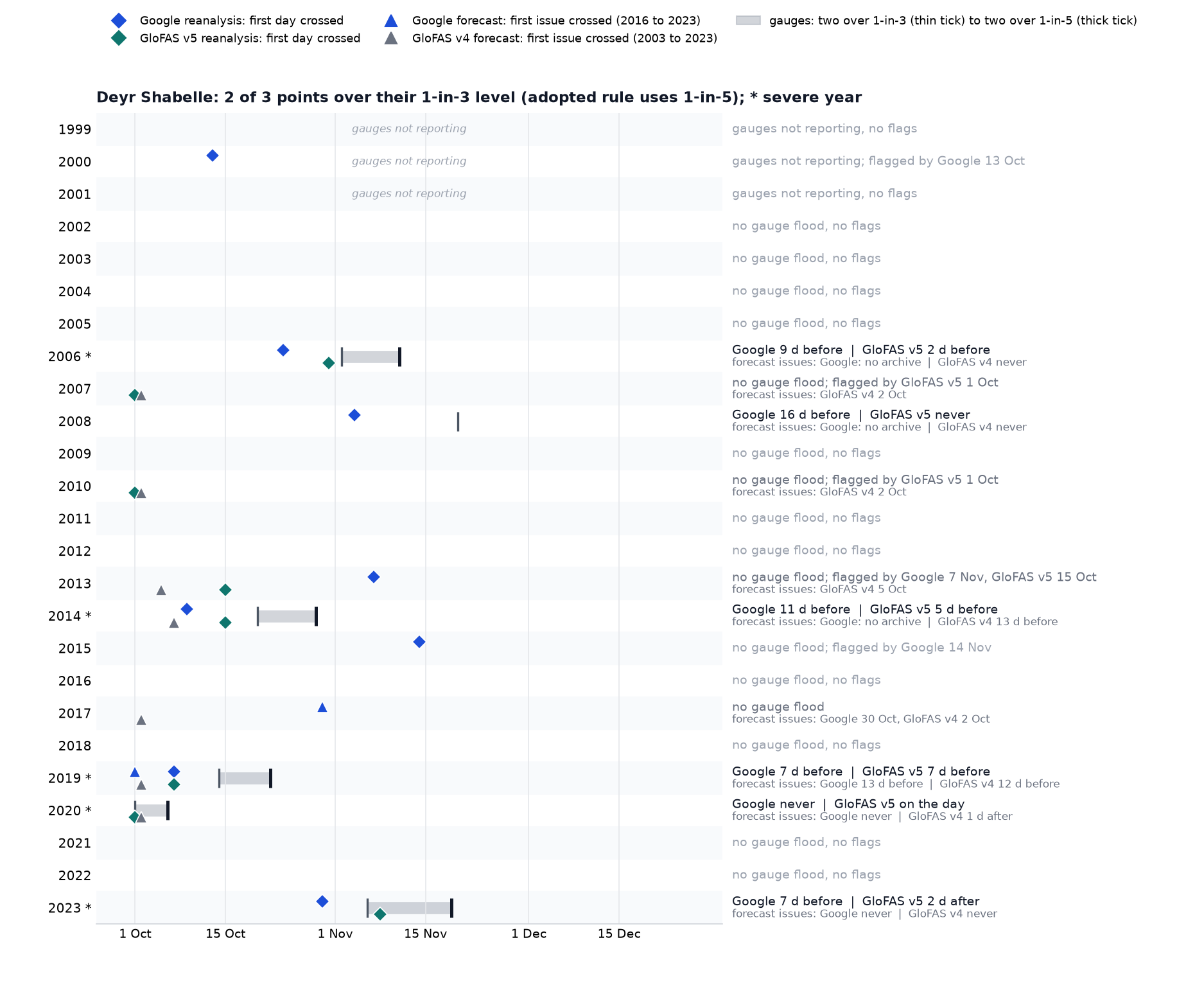
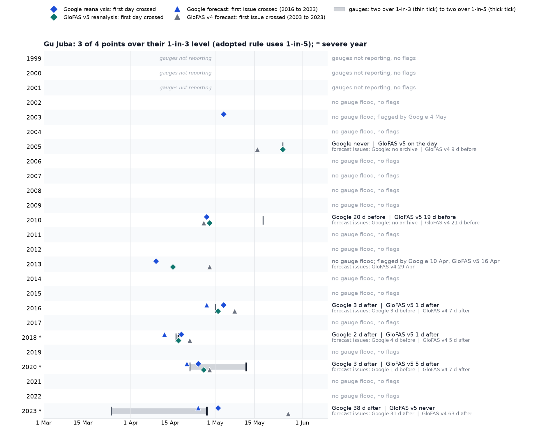
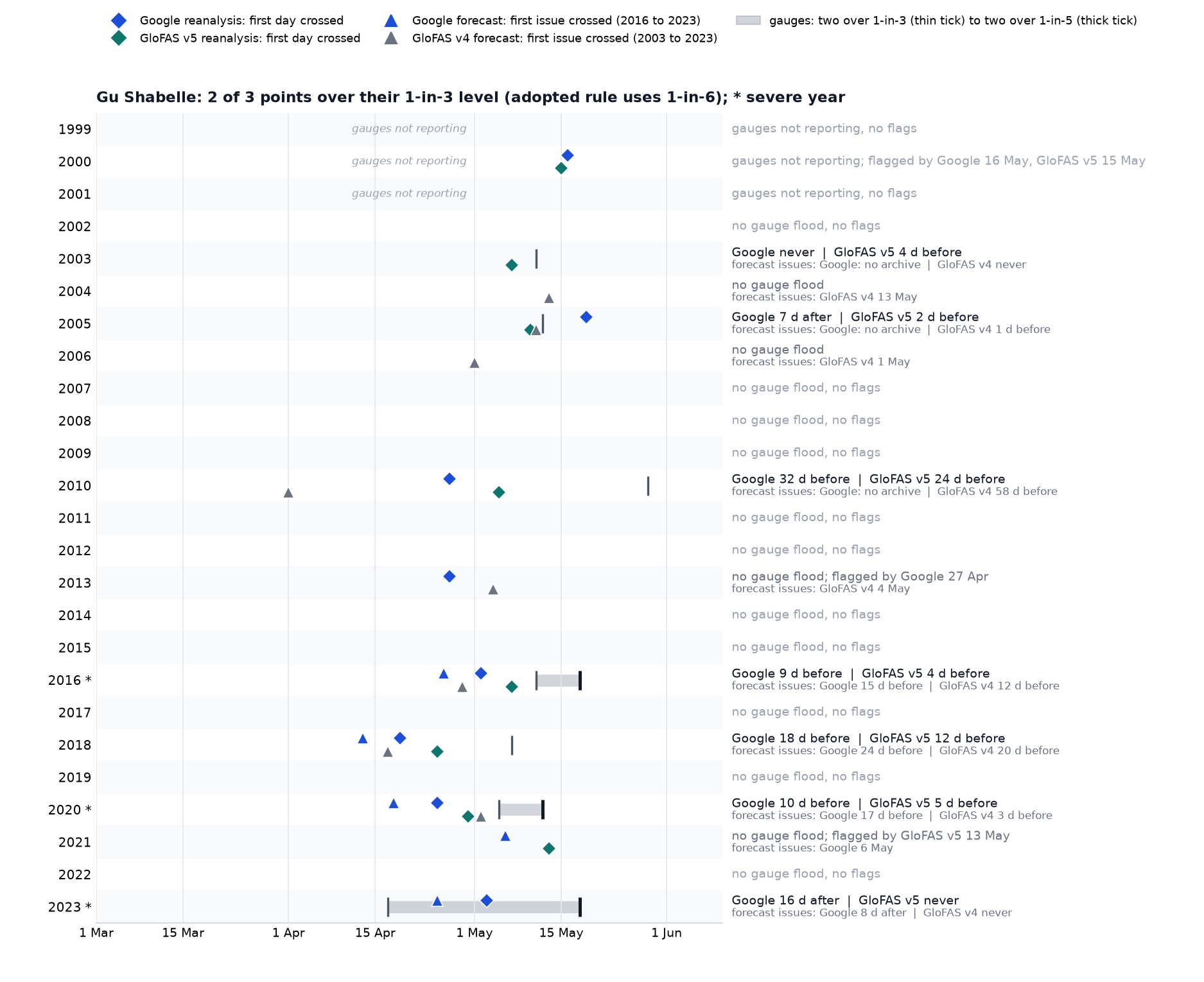
On the Shabelle the models are early. In Deyr, Google crosses in five of the six flood years, 7 to 16 days before onset, and misses 2020; GloFAS v5 crosses in five, between 2 days after and 7 days before, and misses 2008. In Gu, GloFAS v5 crosses in six of seven flood years, all before onset (2 to 24 days); Google crosses in six, four of them before onset (9 to 32 days) and two after. Each model flags one to three of the fifteen or sixteen Shabelle years without a gauge flood. On the Juba the models are late or absent. In Deyr both cross in three of the five flood years, GloFAS v5 1 to 2 days before onset and Google between 4 days after and 5 days before, and each flags four of the eighteen years without a gauge flood. In Gu both cross in five of six flood years but only once before onset (2010); in 2016, 2018 and 2020 they cross 1 to 5 days after, and in 2023 Google crosses more than a month after and GloFAS v5 not at all.
The forecast issues run ahead of the reanalysis on the Shabelle: the Google forecast crossed 15 to 24 days before onset in Gu 2016, 2018 and 2020 and 13 days before in Deyr 2019, and the GloFAS v4 forecast 12 to 13 days before in Deyr 2014 and 2019. On the Juba in Gu the v4 issues come 5 to 7 days after onset in 2016, 2018 and 2020, and the Google issues 1 to 4 days before. Compared with the adopted return periods used in the SWALIM comparison above, 1-in-3 adds a few days of lead on the Shabelle, up to a week for GloFAS v5 in Deyr, at the cost of one to three extra flags per window in years without a gauge flood. On the Juba in Deyr it raises the non-flood flags to four in eighteen years for each model without catching the two remaining flood years.
Every year in a table: dates and leads
Dates are the first day the rule crossed (reanalysis) or the first issue that crossed (forecast), with the lead against the gauges' two-gauge 1-in-3 crossing in brackets where there was one.
| window | year | gauge benchmark | gauges 1-in-3 | gauges 1-in-5 | Google reanalysis | GloFAS v5 reanalysis | Google forecast issue | GloFAS v4 forecast issue |
|---|---|---|---|---|---|---|---|---|
| Deyr Juba | 1999 | not reporting | never | never | no archive | no archive | ||
| Deyr Juba | 2000 | not reporting | never | never | no archive | no archive | ||
| Deyr Juba | 2001 | none | never | never | no archive | no archive | ||
| Deyr Juba | 2002 | none | never | never | no archive | no archive | ||
| Deyr Juba | 2003 | none | never | never | no archive | never | ||
| Deyr Juba | 2004 | none | 27 Nov | 6 Nov | no archive | never | ||
| Deyr Juba | 2005 | none | never | never | no archive | 19 Oct | ||
| Deyr Juba | 2006 * | flood | 30 Oct | 30 Oct | 30 Oct (on the day) | 28 Oct (2 d before) | no archive | 31 Oct (1 d after) |
| Deyr Juba | 2007 | none | never | never | no archive | never | ||
| Deyr Juba | 2008 | flood | 15 Nov | 10 Nov (5 d before) | never | no archive | never | |
| Deyr Juba | 2009 | none | never | never | no archive | never | ||
| Deyr Juba | 2010 | none | never | never | no archive | never | ||
| Deyr Juba | 2011 | none | never | never | no archive | 17 Oct | ||
| Deyr Juba | 2012 | none | never | never | no archive | never | ||
| Deyr Juba | 2013 | none | 18 Nov | never | no archive | never | ||
| Deyr Juba | 2014 * | flood | 22 Oct | 24 Oct | never | never | no archive | 16 Oct (6 d before) |
| Deyr Juba | 2015 | none | 11 Nov | 11 Nov | no archive | 23 Oct | ||
| Deyr Juba | 2016 | none | never | never | never | never | ||
| Deyr Juba | 2017 | flood | 7 Nov | never | 5 Nov (2 d before) | never | 19 Oct (19 d before) | |
| Deyr Juba | 2018 | none | never | 1 Nov | never | never | ||
| Deyr Juba | 2019 | none | 19 Oct | 16 Oct | 12 Oct | never | ||
| Deyr Juba | 2020 | none | never | never | never | never | ||
| Deyr Juba | 2021 | none | never | never | never | never | ||
| Deyr Juba | 2022 | none | never | never | never | never | ||
| Deyr Juba | 2023 * | flood | 25 Oct | 25 Oct | 29 Oct (4 d after) | 24 Oct (1 d before) | never | 10 Oct (15 d before) |
| Deyr Shabelle | 1999 | not reporting | never | never | no archive | no archive | ||
| Deyr Shabelle | 2000 | not reporting | 13 Oct | never | no archive | no archive | ||
| Deyr Shabelle | 2001 | not reporting | never | never | no archive | no archive | ||
| Deyr Shabelle | 2002 | none | never | never | no archive | no archive | ||
| Deyr Shabelle | 2003 | none | never | never | no archive | never | ||
| Deyr Shabelle | 2004 | none | never | never | no archive | never | ||
| Deyr Shabelle | 2005 | none | never | never | no archive | never | ||
| Deyr Shabelle | 2006 * | flood | 2 Nov | 11 Nov | 24 Oct (9 d before) | 31 Oct (2 d before) | no archive | never |
| Deyr Shabelle | 2007 | none | never | 1 Oct | no archive | 2 Oct | ||
| Deyr Shabelle | 2008 | flood | 20 Nov | 4 Nov (16 d before) | never | no archive | never | |
| Deyr Shabelle | 2009 | none | never | never | no archive | never | ||
| Deyr Shabelle | 2010 | none | never | 1 Oct | no archive | 2 Oct | ||
| Deyr Shabelle | 2011 | none | never | never | no archive | never | ||
| Deyr Shabelle | 2012 | none | never | never | no archive | never | ||
| Deyr Shabelle | 2013 | none | 7 Nov | 15 Oct | no archive | 5 Oct | ||
| Deyr Shabelle | 2014 * | flood | 20 Oct | 29 Oct | 9 Oct (11 d before) | 15 Oct (5 d before) | no archive | 7 Oct (13 d before) |
| Deyr Shabelle | 2015 | none | 14 Nov | never | no archive | never | ||
| Deyr Shabelle | 2016 | none | never | never | never | never | ||
| Deyr Shabelle | 2017 | none | never | never | 30 Oct | 2 Oct | ||
| Deyr Shabelle | 2018 | none | never | never | never | never | ||
| Deyr Shabelle | 2019 * | flood | 14 Oct | 22 Oct | 7 Oct (7 d before) | 7 Oct (7 d before) | 1 Oct (13 d before) | 2 Oct (12 d before) |
| Deyr Shabelle | 2020 * | flood | 1 Oct | 6 Oct | never | 1 Oct (on the day) | never | 2 Oct (1 d after) |
| Deyr Shabelle | 2021 | none | never | never | never | never | ||
| Deyr Shabelle | 2022 | none | never | never | never | never | ||
| Deyr Shabelle | 2023 * | flood | 6 Nov | 19 Nov | 30 Oct (7 d before) | 8 Nov (2 d after) | never | never |
| Gu Juba | 1999 | not reporting | never | never | no archive | no archive | ||
| Gu Juba | 2000 | not reporting | never | never | no archive | no archive | ||
| Gu Juba | 2001 | not reporting | never | never | no archive | no archive | ||
| Gu Juba | 2002 | none | never | never | no archive | no archive | ||
| Gu Juba | 2003 | none | 4 May | never | no archive | never | ||
| Gu Juba | 2004 | none | never | never | no archive | never | ||
| Gu Juba | 2005 | flood | 25 May | never | 25 May (on the day) | no archive | 16 May (9 d before) | |
| Gu Juba | 2006 | none | never | never | no archive | never | ||
| Gu Juba | 2007 | none | never | never | no archive | never | ||
| Gu Juba | 2008 | none | never | never | no archive | never | ||
| Gu Juba | 2009 | none | never | never | no archive | never | ||
| Gu Juba | 2010 | flood | 18 May | 28 Apr (20 d before) | 29 Apr (19 d before) | no archive | 27 Apr (21 d before) | |
| Gu Juba | 2011 | none | never | never | no archive | never | ||
| Gu Juba | 2012 | none | never | never | no archive | never | ||
| Gu Juba | 2013 | none | 10 Apr | 16 Apr | no archive | 29 Apr | ||
| Gu Juba | 2014 | none | never | never | no archive | never | ||
| Gu Juba | 2015 | none | never | never | no archive | never | ||
| Gu Juba | 2016 | flood | 1 May | 4 May (3 d after) | 2 May (1 d after) | 28 Apr (3 d before) | 8 May (7 d after) | |
| Gu Juba | 2017 | none | never | never | never | never | ||
| Gu Juba | 2018 * | flood | 17 Apr | 18 Apr | 19 Apr (2 d after) | 18 Apr (1 d after) | 13 Apr (4 d before) | 22 Apr (5 d after) |
| Gu Juba | 2019 | none | never | never | never | never | ||
| Gu Juba | 2020 * | flood | 22 Apr | 12 May | 25 Apr (3 d after) | 27 Apr (5 d after) | 21 Apr (1 d before) | 29 Apr (7 d after) |
| Gu Juba | 2021 | none | never | never | never | never | ||
| Gu Juba | 2022 | none | never | never | never | never | ||
| Gu Juba | 2023 * | flood | 25 Mar | 28 Apr | 2 May (38 d after) | never | 25 Apr (31 d after) | 27 May (63 d after) |
| Gu Shabelle | 1999 | not reporting | never | never | no archive | no archive | ||
| Gu Shabelle | 2000 | not reporting | 16 May | 15 May | no archive | no archive | ||
| Gu Shabelle | 2001 | not reporting | never | never | no archive | no archive | ||
| Gu Shabelle | 2002 | none | never | never | no archive | no archive | ||
| Gu Shabelle | 2003 | flood | 11 May | never | 7 May (4 d before) | no archive | never | |
| Gu Shabelle | 2004 | none | never | never | no archive | 13 May | ||
| Gu Shabelle | 2005 | flood | 12 May | 19 May (7 d after) | 10 May (2 d before) | no archive | 11 May (1 d before) | |
| Gu Shabelle | 2006 | none | never | never | no archive | 1 May | ||
| Gu Shabelle | 2007 | none | never | never | no archive | never | ||
| Gu Shabelle | 2008 | none | never | never | no archive | never | ||
| Gu Shabelle | 2009 | none | never | never | no archive | never | ||
| Gu Shabelle | 2010 | flood | 29 May | 27 Apr (32 d before) | 5 May (24 d before) | no archive | 1 Apr (58 d before) | |
| Gu Shabelle | 2011 | none | never | never | no archive | never | ||
| Gu Shabelle | 2012 | none | never | never | no archive | never | ||
| Gu Shabelle | 2013 | none | 27 Apr | never | no archive | 4 May | ||
| Gu Shabelle | 2014 | none | never | never | no archive | never | ||
| Gu Shabelle | 2015 | none | never | never | no archive | never | ||
| Gu Shabelle | 2016 * | flood | 11 May | 18 May | 2 May (9 d before) | 7 May (4 d before) | 26 Apr (15 d before) | 29 Apr (12 d before) |
| Gu Shabelle | 2017 | none | never | never | never | never | ||
| Gu Shabelle | 2018 | flood | 7 May | 19 Apr (18 d before) | 25 Apr (12 d before) | 13 Apr (24 d before) | 17 Apr (20 d before) | |
| Gu Shabelle | 2019 | none | never | never | never | never | ||
| Gu Shabelle | 2020 * | flood | 5 May | 12 May | 25 Apr (10 d before) | 30 Apr (5 d before) | 18 Apr (17 d before) | 2 May (3 d before) |
| Gu Shabelle | 2021 | none | never | 13 May | 6 May | never | ||
| Gu Shabelle | 2022 | none | never | never | never | never | ||
| Gu Shabelle | 2023 * | flood | 17 Apr | 18 May | 3 May (16 d after) | never | 25 Apr (8 d after) | never |
An observational fallback: bank full at the gauges
SWALIM publishes an official bank-full level for each gauge, the reading at which the river tops its banks (Juba: Dollow 6.0 m, Luuq 7.0 m, Bardheere 10.4 m, Bualle 12.0 m; Shabelle: Belet Weyne 8.3 m, Bulo Burti 8.0 m, Jowhar 5.5 m), and a high-risk level below it. This section scores an observational trigger set at those levels, on its own and as a fallback that releases funds when no forecast window has activated. Two limits apply. The gauge record is capped at bank full, so a reading at bank full means at least bank full. Bardheere's official bank-full level (10.4 m) is above the highest reading in its record (8.0 m), so that gauge can never reach it.

Every season in a table: dates, stations and lags
| window | year | benchmark | gauges: two over 1-in-3 | forecast trigger first day | two gauges at the high-risk level | first gauge at bank full | two gauges at bank full |
|---|---|---|---|---|---|---|---|
| Deyr Juba | 2006 | severe | 30 Oct 1-in-5: 30 Oct | 29 Oct | 28 Oct (Luuq, Bardheere) | no | no |
| Deyr Juba | 2008 | flood | 15 Nov 1-in-5: no | never | no | no | no |
| Deyr Juba | 2011 | none | no 1-in-5: no | never | 2 Dec (Luuq, Bardheere) | no | no |
| Deyr Juba | 2014 | severe | 22 Oct 1-in-5: 24 Oct | never | 24 Oct (Luuq, Bardheere) | no | no |
| Deyr Juba | 2017 | flood | 7 Nov 1-in-5: no | never | 7 Nov (Dollow, Bardheere) | no | no |
| Deyr Juba | 2019 | none | no 1-in-5: no | never | 9 Oct (Dollow, Bardheere) | no | no |
| Deyr Juba | 2022 | none | no 1-in-5: no | never | 30 Oct (Dollow, Bardheere) | no | no |
| Deyr Juba | 2023 | severe | 25 Oct 1-in-5: 25 Oct | 29 Oct | 22 Oct (Luuq, Bardheere) | 3 Nov (Dollow, Luuq) 5 d after the trigger; 9 d after 1-in-5 | 3 Nov (Dollow, Luuq) |
| Deyr Shabelle | 2006 | severe | 2 Nov 1-in-5: 11 Nov | 2 Nov | 11 Nov (Belet Weyne, Bulo Burti) | 10 Nov (Belet Weyne) 8 d after the trigger; 1 d before 1-in-5 | no |
| Deyr Shabelle | 2008 | flood | 20 Nov 1-in-5: no | never | no | no | no |
| Deyr Shabelle | 2014 | severe | 20 Oct 1-in-5: 29 Oct | 17 Oct | 24 Oct (Belet Weyne, Jowhar) | no | no |
| Deyr Shabelle | 2015 | none | no 1-in-5: no | never | no | 25 Oct (Jowhar) trigger never crossed; no 1-in-5 crossing | no |
| Deyr Shabelle | 2019 | severe | 14 Oct 1-in-5: 22 Oct | 13 Oct | 19 Oct (Belet Weyne, Jowhar) | 25 Oct (Belet Weyne) 12 d after the trigger; 3 d after 1-in-5 | 8 Nov (Belet Weyne, Bulo Burti) |
| Deyr Shabelle | 2020 | severe | 1 Oct 1-in-5: 6 Oct | never | 1 Oct (Belet Weyne, Bulo Burti) | no | no |
| Deyr Shabelle | 2023 | severe | 6 Nov 1-in-5: 19 Nov | 10 Nov | 19 Nov (Belet Weyne, Bulo Burti) | 12 Nov (Belet Weyne) 2 d after the trigger; 7 d before 1-in-5 | 22 Nov (Belet Weyne, Bulo Burti) |
| Gu Juba | 2005 | flood | 25 May 1-in-5: no | never | no | no | no |
| Gu Juba | 2010 | flood | 18 May 1-in-5: no | never | no | no | no |
| Gu Juba | 2013 | none | no 1-in-5: no | 12 Apr | no | no | no |
| Gu Juba | 2016 | flood | 1 May 1-in-5: no | 7 May | 7 May (Dollow, Luuq) | no | no |
| Gu Juba | 2018 | severe | 17 Apr 1-in-5: 18 Apr | 20 Apr | 18 Apr (Luuq, Bardheere) | no | no |
| Gu Juba | 2020 | severe | 22 Apr 1-in-5: 12 May | 29 Apr | 1 May (Dollow, Bardheere) | no | no |
| Gu Juba | 2023 | severe | 25 Mar 1-in-5: 28 Apr | never | 24 Mar (Dollow, Bardheere) | no | no |
| Gu Shabelle | 2003 | flood | 11 May 1-in-5: no | never | no | no | no |
| Gu Shabelle | 2005 | flood | 12 May 1-in-5: no | never | 12 May (Belet Weyne, Bulo Burti) | no | no |
| Gu Shabelle | 2010 | flood | 29 May 1-in-5: no | never | 12 May (Belet Weyne, Jowhar) | no | no |
| Gu Shabelle | 2013 | none | no 1-in-5: no | 6 May | no | no | no |
| Gu Shabelle | 2015 | none | no 1-in-5: no | never | no | 20 Apr (Jowhar) trigger never crossed; no 1-in-5 crossing | no |
| Gu Shabelle | 2016 | severe | 11 May 1-in-5: 18 May | 12 May | 10 May (Belet Weyne, Jowhar) | 18 May (Belet Weyne) 6 d after the trigger; same day as 1-in-5 | no |
| Gu Shabelle | 2018 | flood | 7 May 1-in-5: no | 5 May | 9 May (Belet Weyne, Bulo Burti) | no | no |
| Gu Shabelle | 2020 | severe | 5 May 1-in-5: 12 May | 30 Apr | 5 May (Belet Weyne, Jowhar) | 12 May (Belet Weyne) 12 d after the trigger; same day as 1-in-5 | 29 May (Belet Weyne, Bulo Burti) |
| Gu Shabelle | 2021 | none | no 1-in-5: no | never | no | 26 May (Belet Weyne) trigger never crossed; no 1-in-5 crossing | no |
| Gu Shabelle | 2023 | severe | 17 Apr 1-in-5: 18 May | never | 23 May (Belet Weyne, Bulo Burti) | 9 May (Belet Weyne) trigger never crossed; 9 d before 1-in-5 | 25 May (Belet Weyne, Bulo Burti) |
Where a gauge reached bank full in a benchmark flood, it did so between 9 days before and 9 days after the 1-in-5 crossing: Deyr Shabelle 2006, 2019 and 2023 at 1 day before, 3 days after and 7 days before; Gu Shabelle 2016 and 2020 on the day and Gu Shabelle 2023 at 9 days before; Deyr Juba 2023 at 9 days after. In every one of those seasons except Gu 2023 on the Shabelle the forecast trigger had already crossed, 2 to 12 days earlier. No Juba gauge has read bank full in Gu in the record. Bank full confirms a flood; it does not warn of one.
Behind the adopted trigger the fallback recovers one benchmark season, Gu 2023 on the Shabelle (Belet Weyne at bank full on 9 May, 9 days before the gauges crossed 1-in-5 on 18 May). It adds three seasons the two-gauge benchmark does not call floods: Deyr 2015 and Gu 2015 on the Shabelle, and Gu 2021 at Belet Weyne. All three had flooding. Gu 2021 is the flood the benchmark misses because the gauge is censored at bank full; SWALIM reported flooding upstream of Belet Weyne and EM-DAT records 400,000 people affected. In both 2015 seasons SWALIM issued high-risk watches or a Flood Alert, with floods reported at Jamame and Jilib. The fallback would therefore have released funds in four seasons the forecast trigger did not (Gu 2015, Deyr 2015, Gu 2021 and Gu 2023, all on the Shabelle), each time at or after the point where the river was already over its banks. In 2015 and 2021 no window activated at all, so the envelope's activation rate would rise from 8 to 10 years in 25, about 1-in-2.6.
The high-risk level is too loose to release funds on its own. Two Juba gauges at the high-risk level occurs in seven Deyr seasons (2006, 2011, 2014, 2017, 2019, 2022, 2023), three of them (2011, 2019, 2022) in seasons without a two-gauge flood. Two Shabelle gauges at the high-risk level in Deyr matches the five severe years exactly; in Gu it adds 2005, 2010 and 2018. It is the level at which SWALIM's own bulletins escalate, and the SWALIM section above shows that step arriving 1 to 7 days before onset in six of the twelve seasons with a bulletin and a gauge event. On this record the fallback would be: bank full at any monitored gauge releases the action funds when no forecast window has activated, and two gauges at the high-risk level counts as a readiness signal, not a release. SWALIM publishes the gauge readings daily with about a day's delay, so the fallback's lead is zero or negative. It covers floods the models miss; it does not add lead time.
Open items before a trigger report
- Impact years are still undefined. The trigger is scored against gauge levels, not against recorded humanitarian impact. Until impact years exist, severe-year coverage is a proxy.
- The reanalysis cannot pick the model. Many assignments tie, so the model per window rests on lead-time skill and on operational considerations, not on the backtest.
- Google cannot be calibrated on its own forecasts. Its reforecast starts in 2016, and a 1-in-3 threshold needs about 12 years, so a Google window is necessarily calibrated on the retrospective and only checked at lead time.
- Two Juba points can no longer be verified. Bardheere's gauge record ends 2023-11-30 and Bualle's 2024-03-14. Both can still be forecast at, but neither can be checked against observations from here on.
- Readiness coverage is low in both seasons, which is accepted rather than solved: at 8 to 12 days the GloFAS v4 median led 2 of the 8 Gu window activations and 2 of the 6 Deyr ones, so an activation may arrive with no readiness phase.