edge-extend

Usage¶

topo-tools edge-extend example.geojson

from topo_tools import edge_extend

edge_extend("example.geojson", "example_extended.geojson")

OUTPUT_FILE (positional, optional) defaults to INPUT_FILE with an _extended suffix.

# Explicit output
topo-tools edge-extend example.gpkg example_extended.gpkg

# Rerun and overwrite a previous output
topo-tools edge-extend example.parquet example_extended.parquet --overwrite

Polygons the size of small countries typically take a few seconds; larger ones at full detail finish in about 10 min. Processing time is proportional to total perimeter length rather than area. The spacing between points on a line is chosen automatically per file: the source data's own level of detail (via each file's median real segment length) sets a finer starting point when it's naturally detailed, never coarser than the fixed default otherwise. See docs/explanation/voronoi-memory.md for why this no longer depends on a memory budget.

Run topo-tools edge-extend --help for the full, always-current option list.

How it Works¶

edge-extend applies the Voronoi algorithm along polygon edges, giving results similar to a euclidean allocation raster. Unlike euclidean allocation, the source is never transformed from vector to raster. All internal polygon topology remains unchanged, with the exception of internal holes, which are filled the same way the exterior is filled out.

The overall processing can be broken down into 4 distinct types of geometry transformations:

• make lines from polygons
• make points from lines
• make voronoi from points
• merge polygons with voronoi

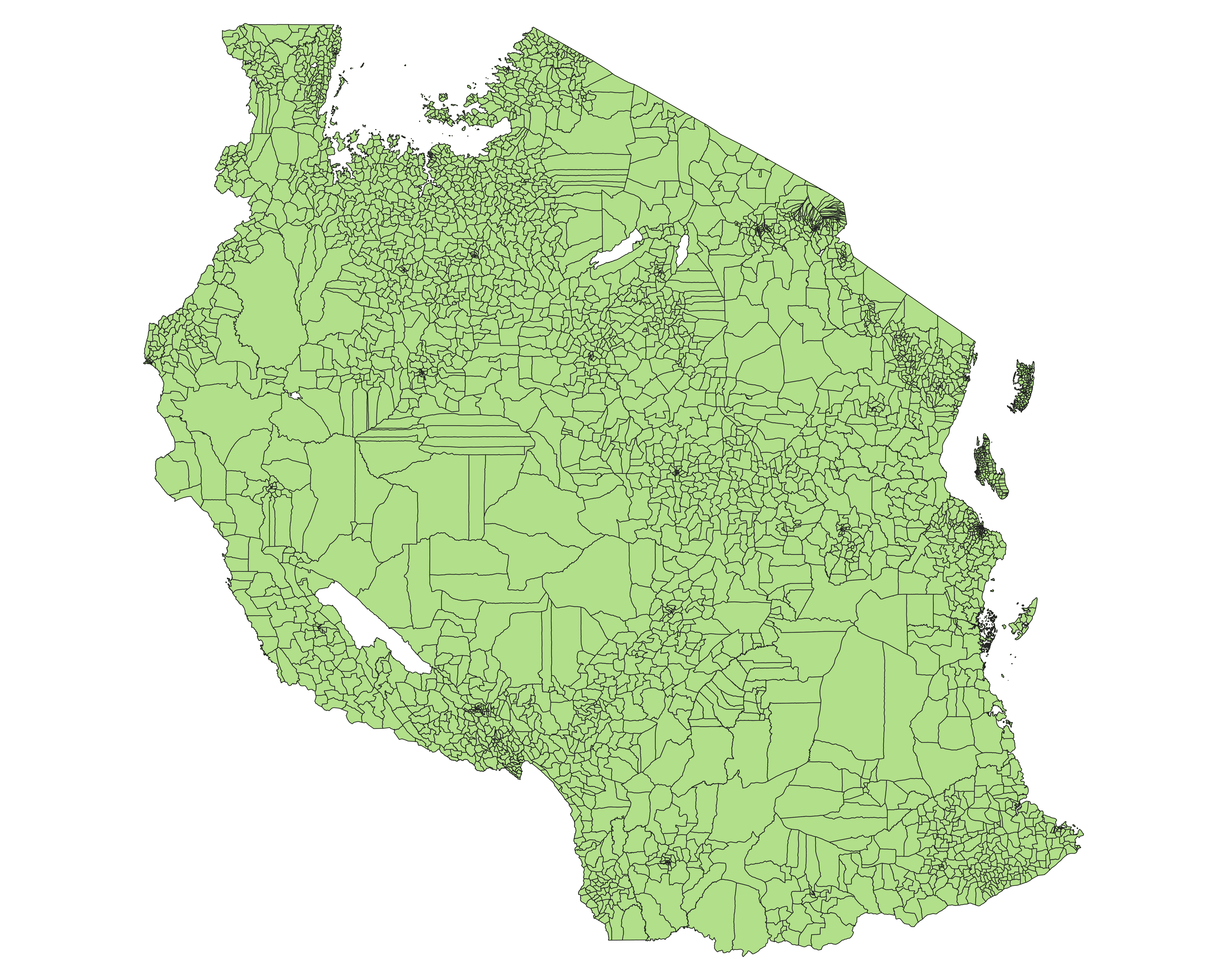
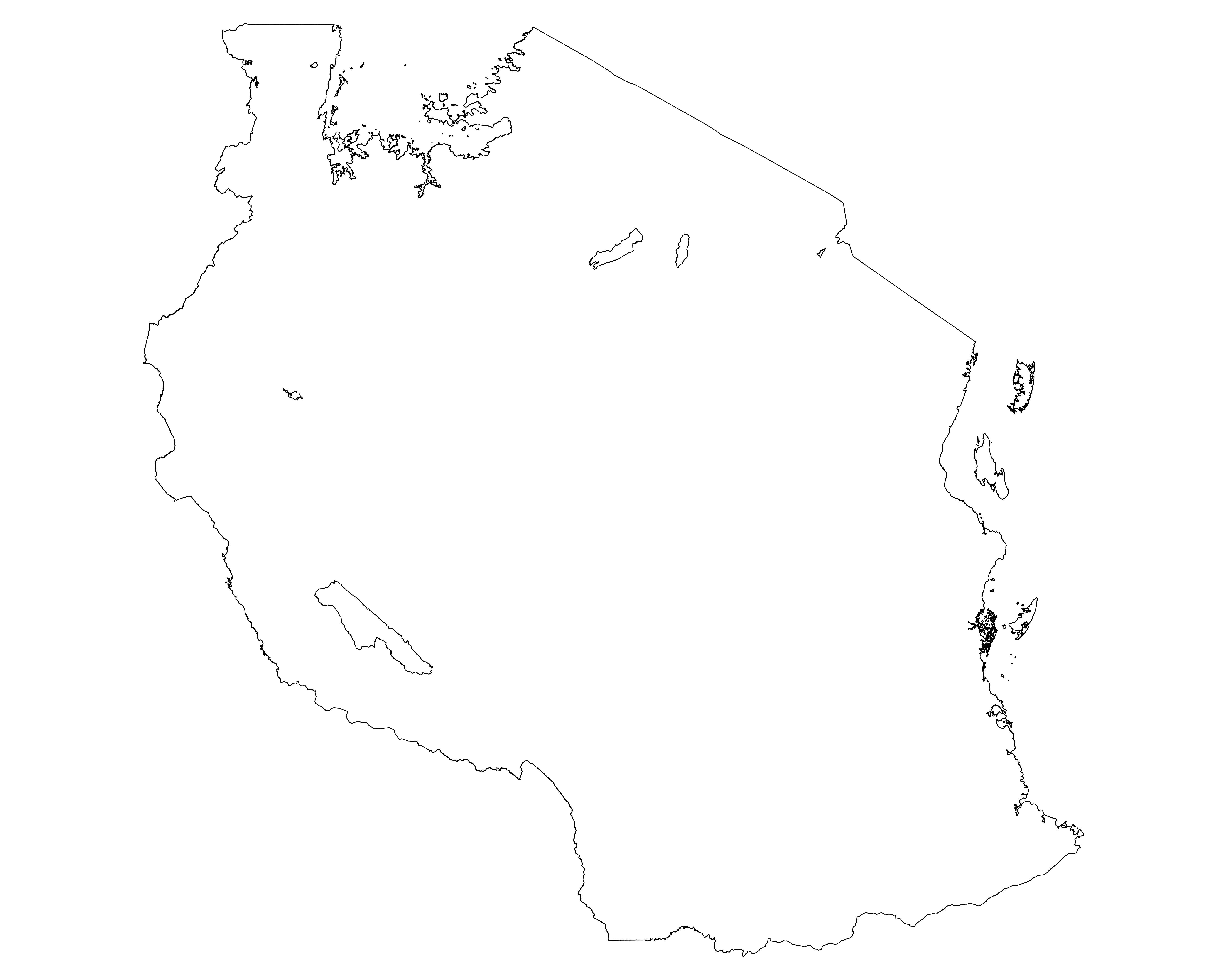
Polygon to Line: The first part extracts outlines from the polygon, first by dissolving all polygons together, then by taking the intersection between the outline of the dissolved and the original layer. By intersecting these two together, it retains attribute information of where segments originate from.

Original Input	Outlines

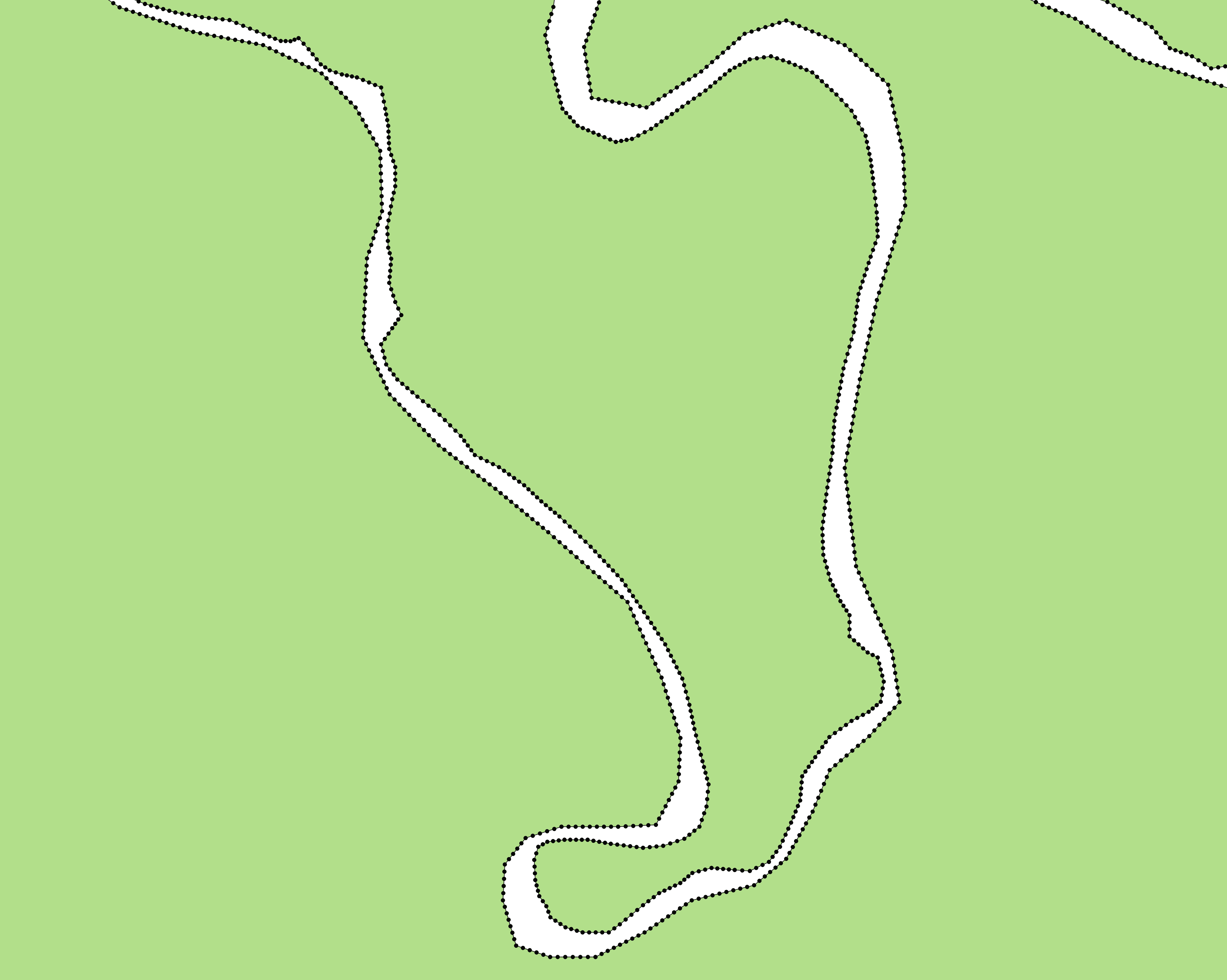
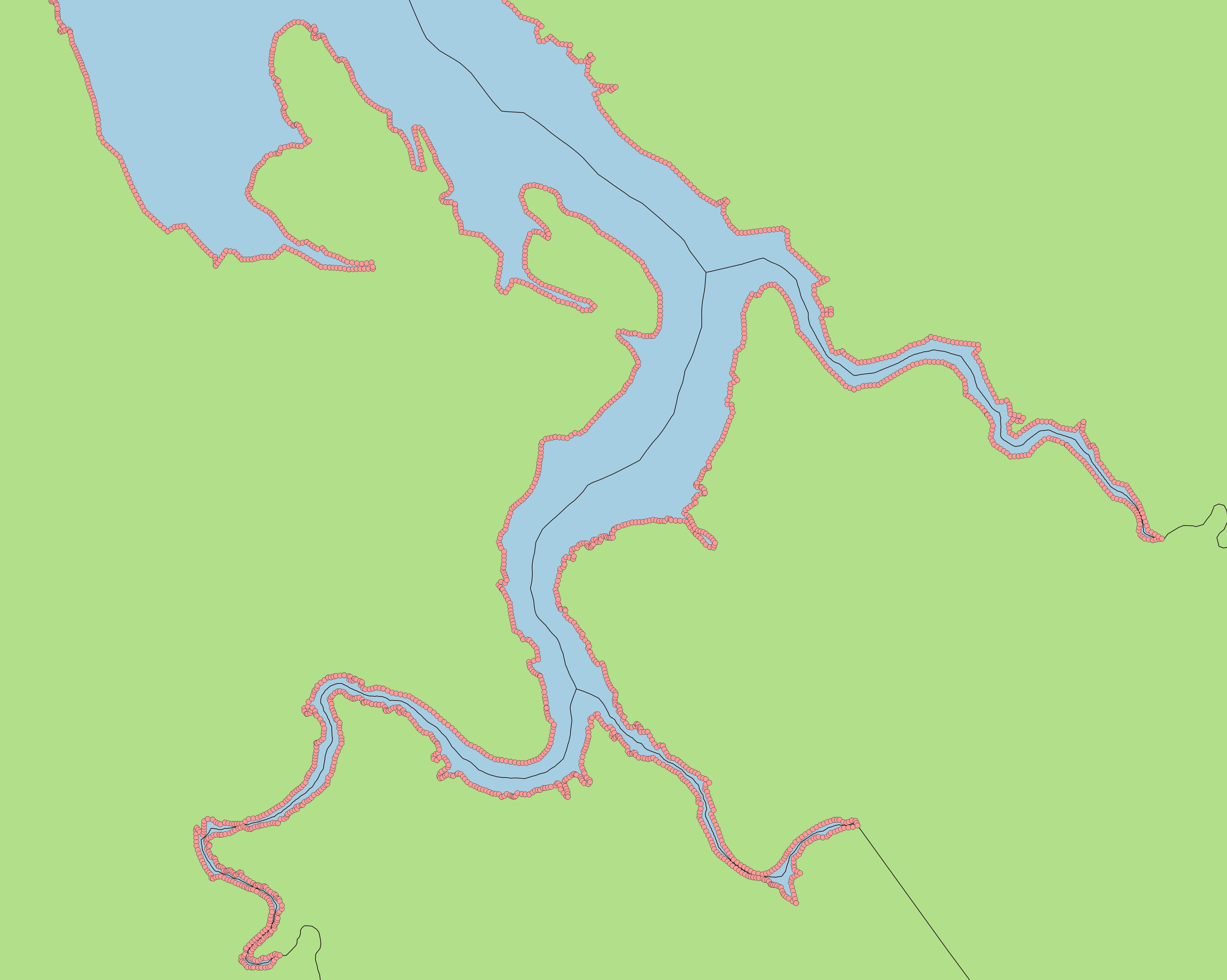
Line to Point: Lines are converted to points using two methods. The first set of points are taken from all vertices that make up a line. However, for certain areas like winding rivers and deltas, this in an insufficient level of detail to properly center the resulting voronoi. With just vertices, the center lines would zigzag through gaps instead of going straight through them. Lines are therefore split up into segments based on an automatically-chosen distance, with points taken at the breaks between segments.

Points along River	Final Result along Delta

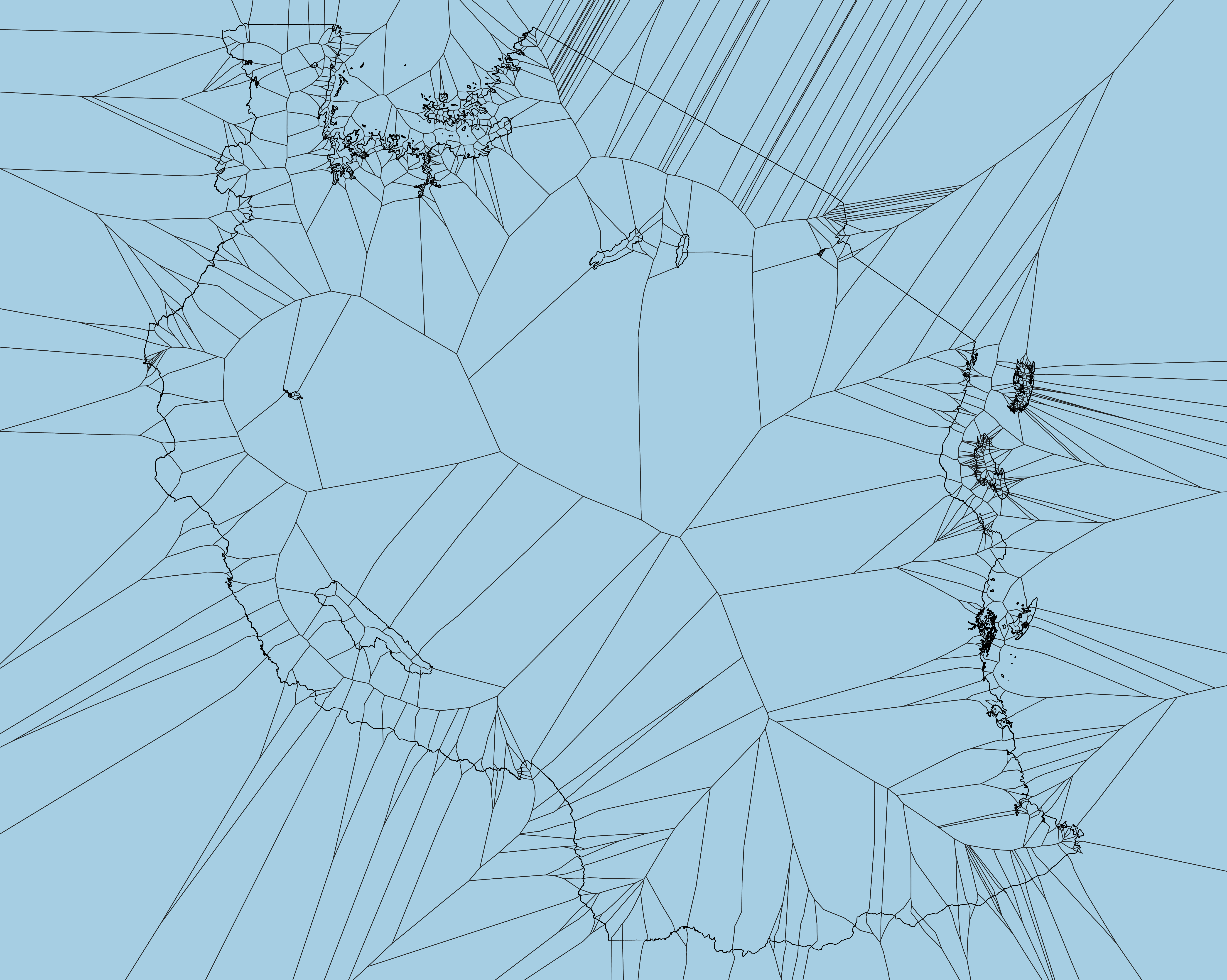
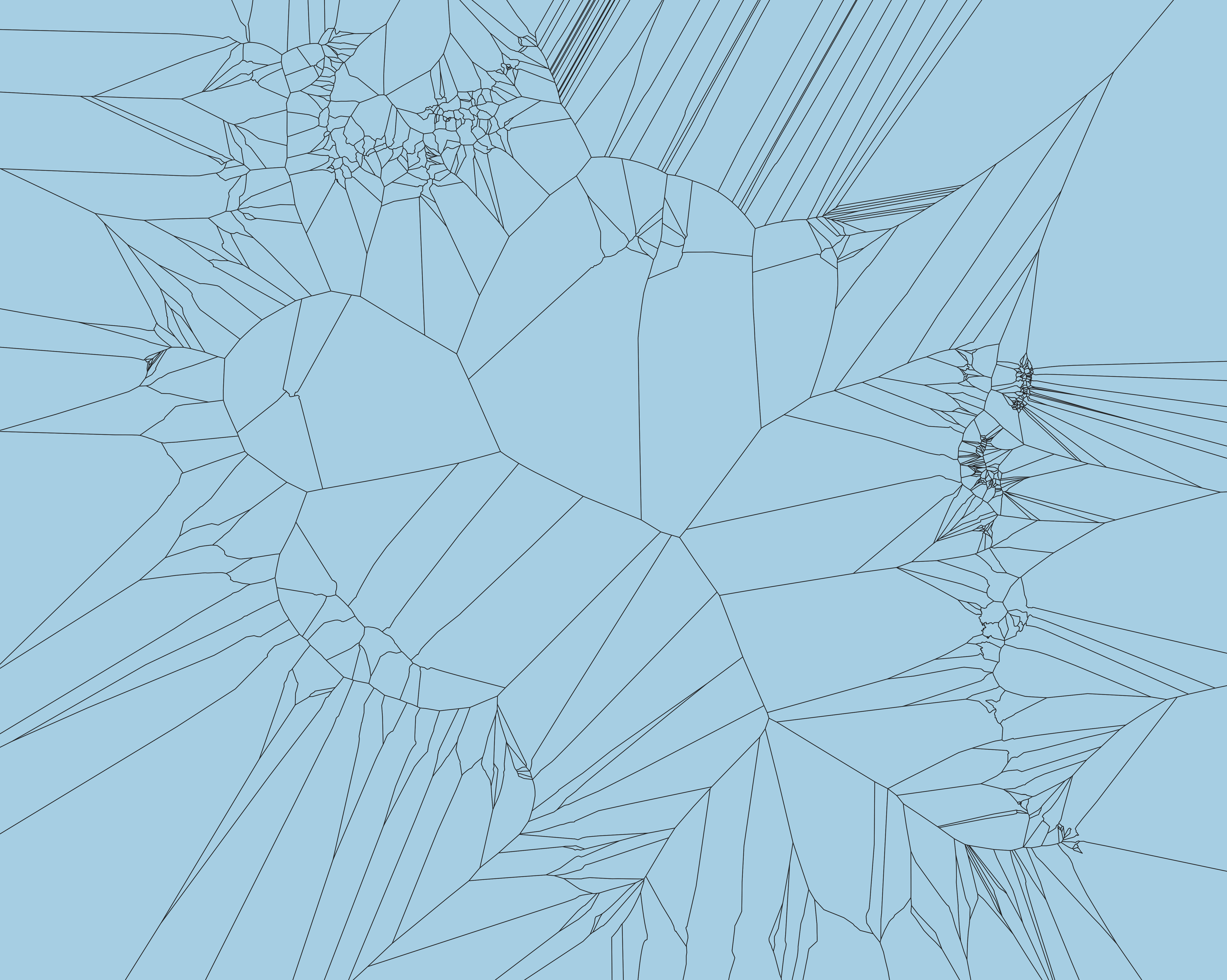
Point to Voronoi: For country sized inputs, there may be hundreds of thousands, if not millions of individual voronoi polygons created in this step. Because each individual section retains attribute information of what polygon it originated from, they can be dissolved together to a simplified output.

Points with Voronoi	Voronoi Only

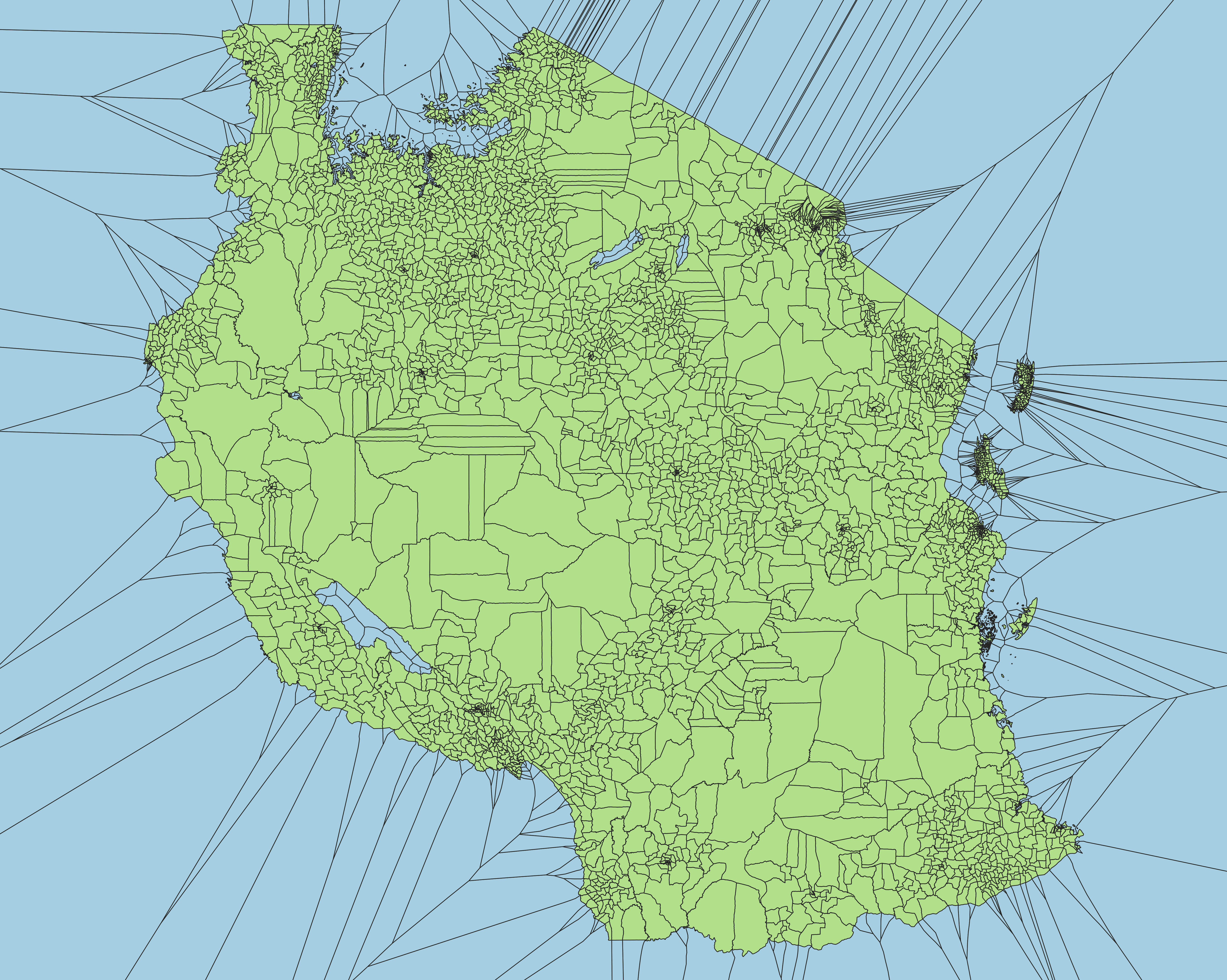
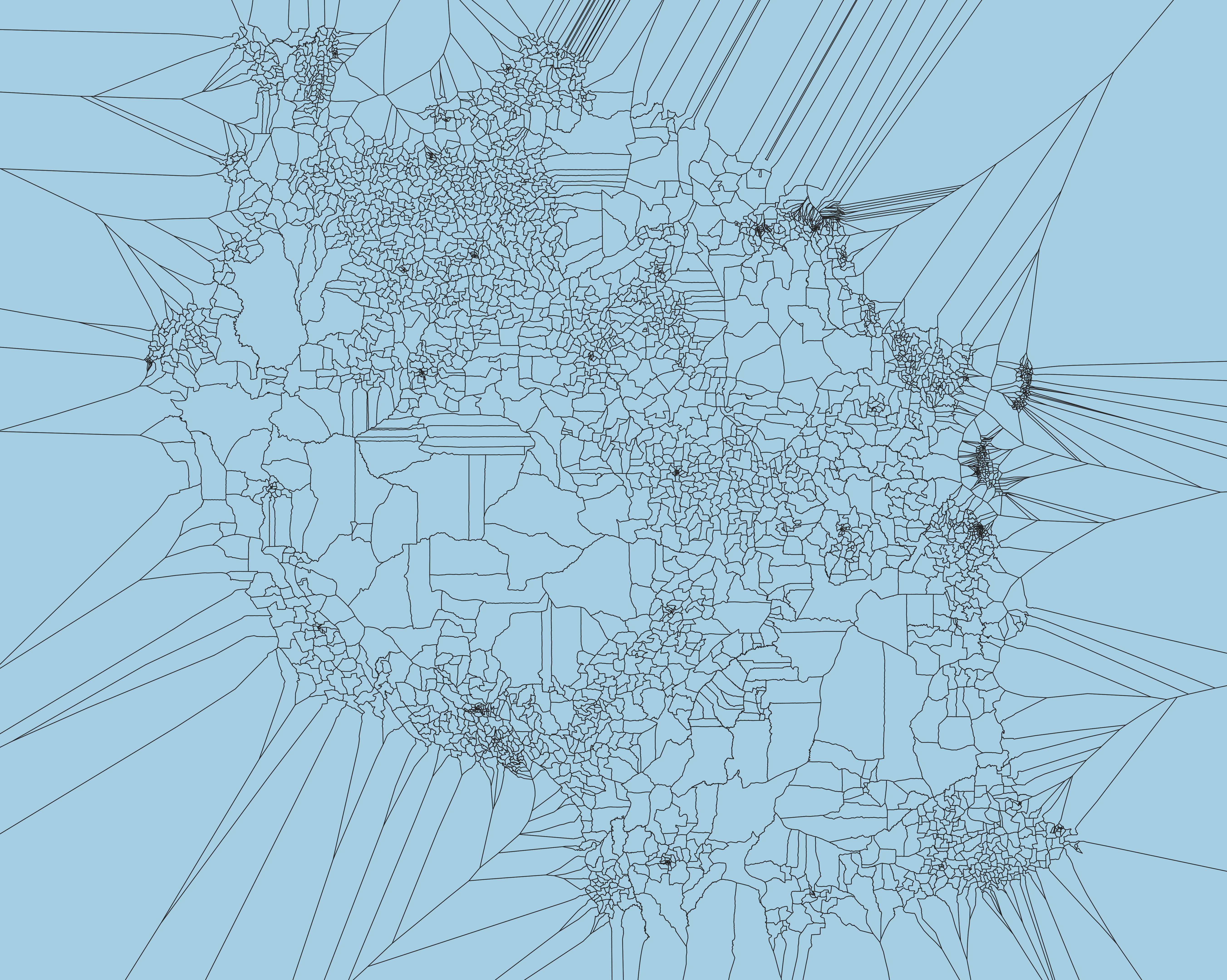
Polygon-Voronoi Merge: The original polygon is overlayed in a union with the voronoi. Boundaries from the inner area are kept from the original, dissolved with polygons containing matching attributes from the outside area. The dissolved layer is the final output of the tool.

Original over Voronoi	Final Output

Correctness Guards¶

The pipeline raises rather than silently producing a wrong result: the point-to-Voronoi stage raises if its shared-boundary-zone difference drops any fid entirely, and the final merge stage raises if any fid's extended geometry no longer covers its own original footprint. See docs/adr/0090-bbox-prefilter-shared-boundary-zone-difference.md and docs/explanation/voronoi-memory.md.

Use Case 1: Matching sub-national boundary (ADM3) to national (ADM0)¶

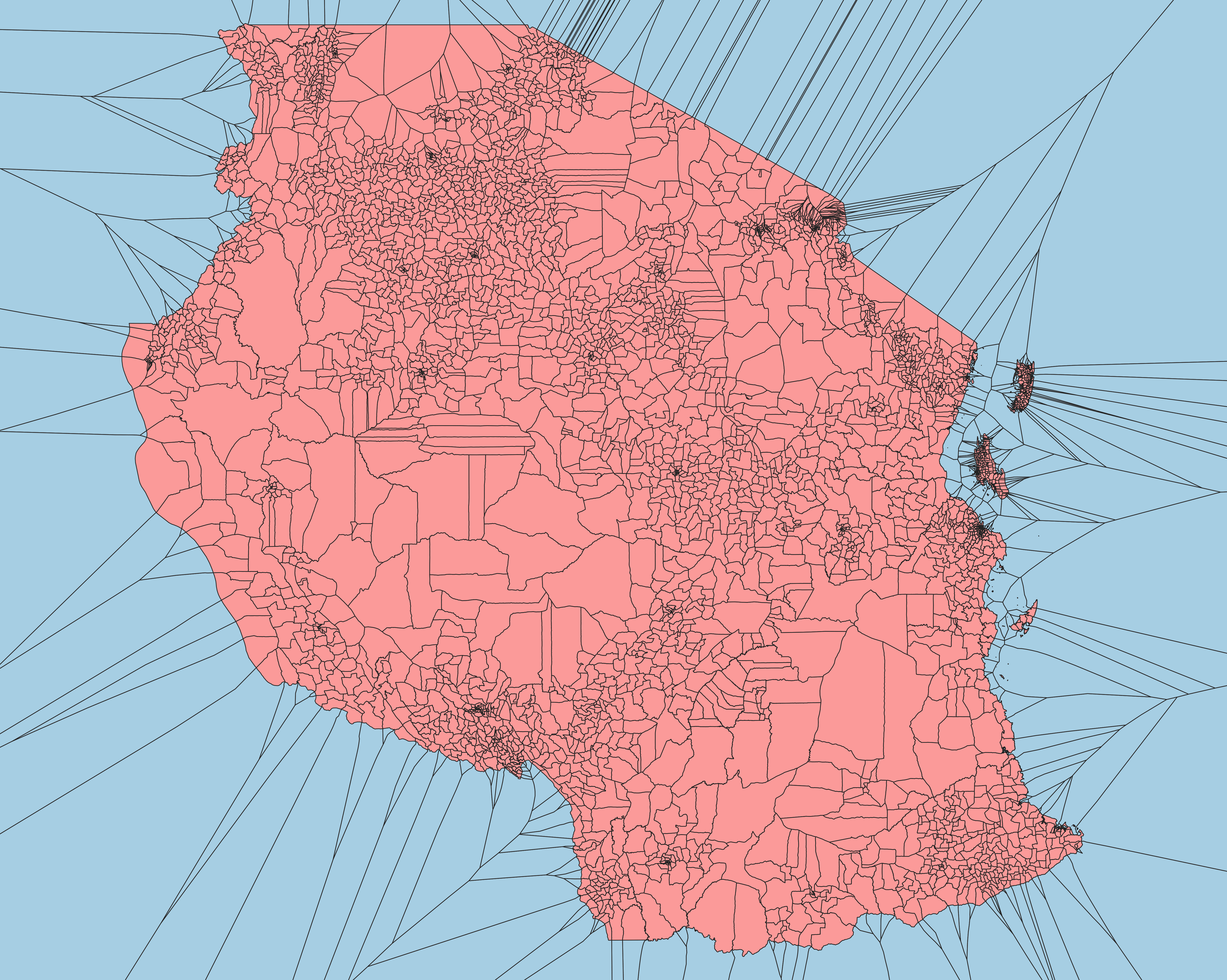
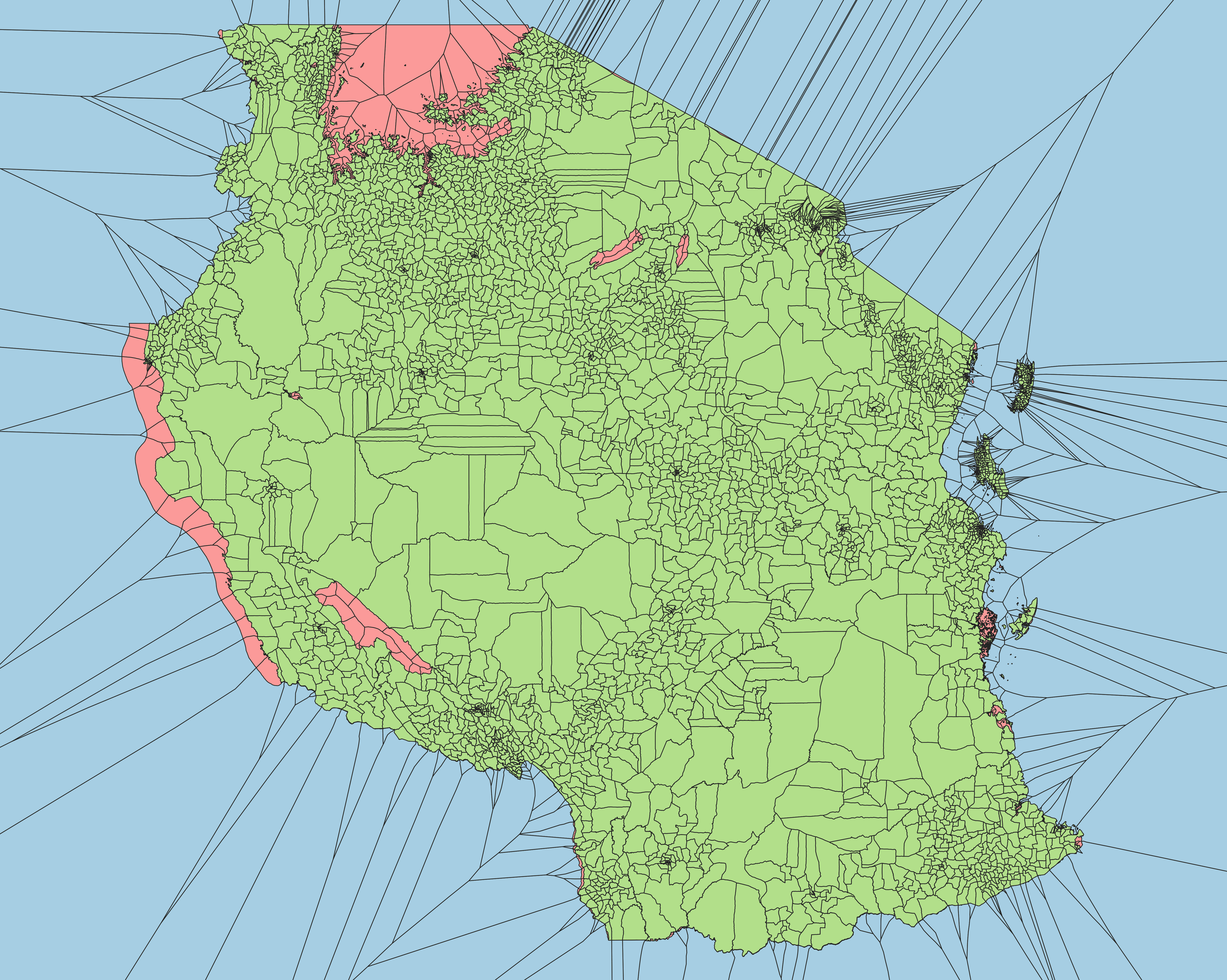
One original use case for this tool was resolving edge differences between different levels of administrative boundaries, where some layers included water bodies but others did not. The United Republic of Tanzania is used in this example as it contains many elements that have been difficult to resolve in the past: lakes along international boundaries, internal water bodies shared by multiple areas, groups of islands, etc. The diagram on the left shows how the ADM3 layer would appear in a global edge-matched geodatabase. The diagram on the right shows how water areas are allocated compared to the original.

ADM0 over Voronoi	Original vs ADM0 edges

Use Case 2: Topologically clean international boundaries¶

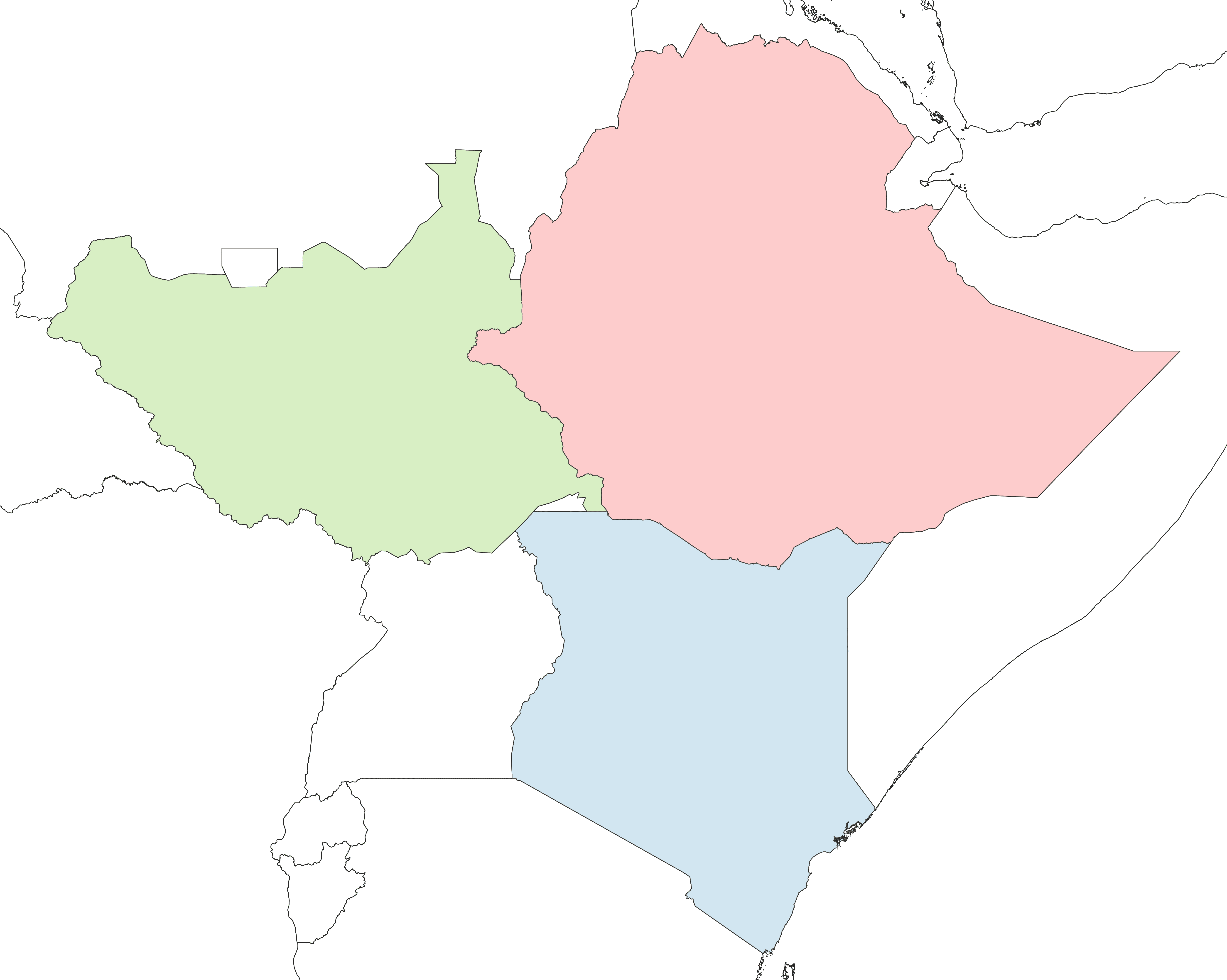
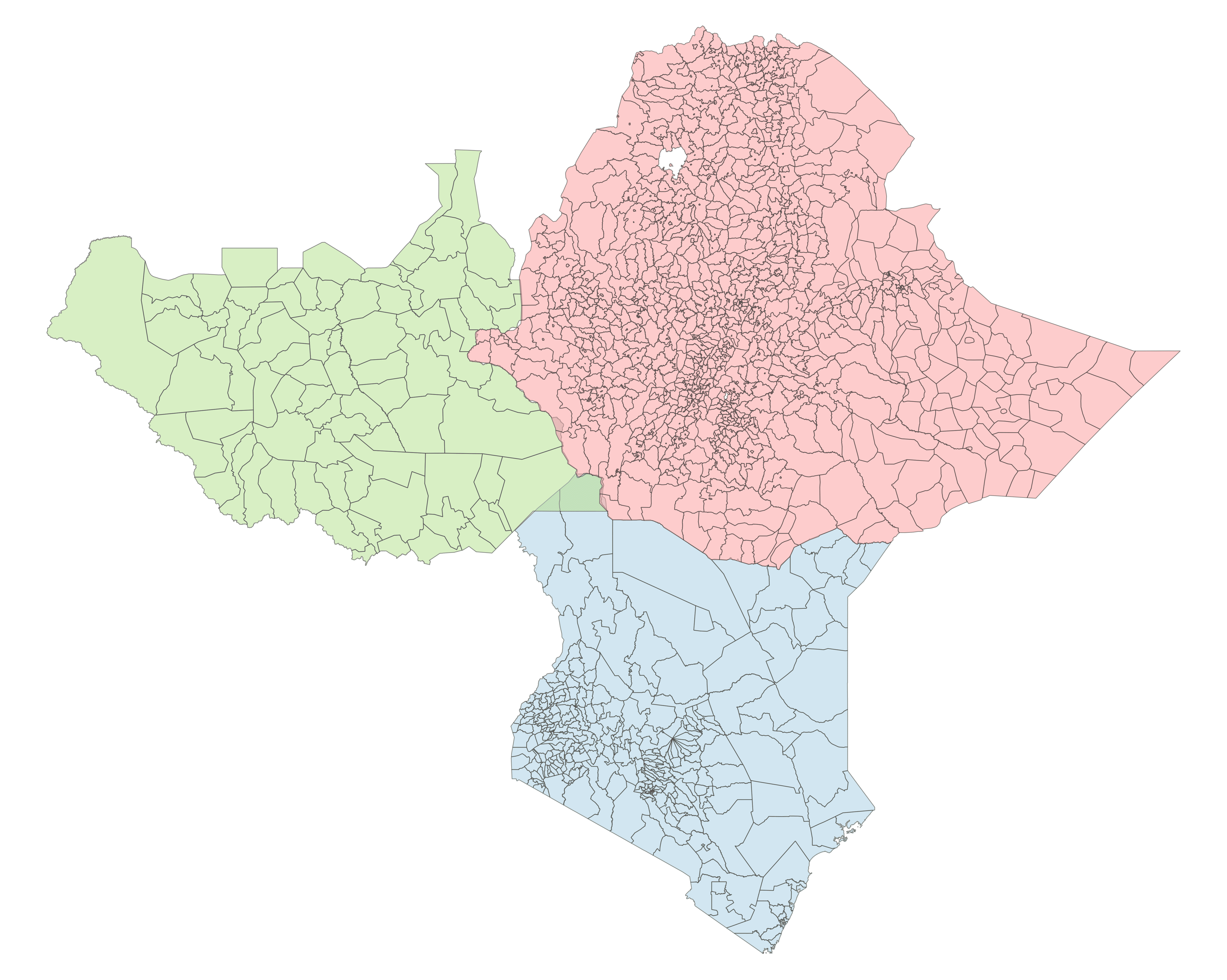
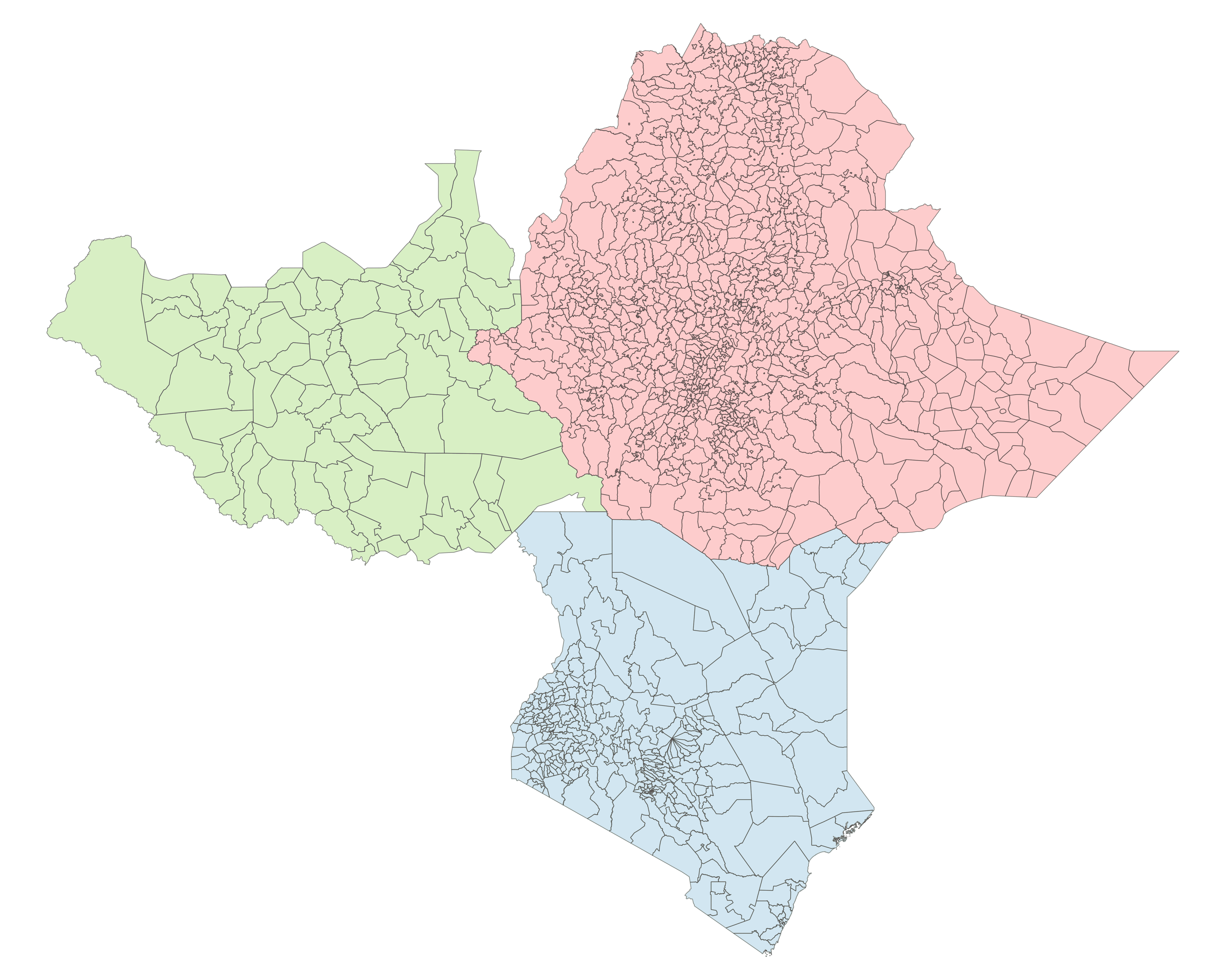
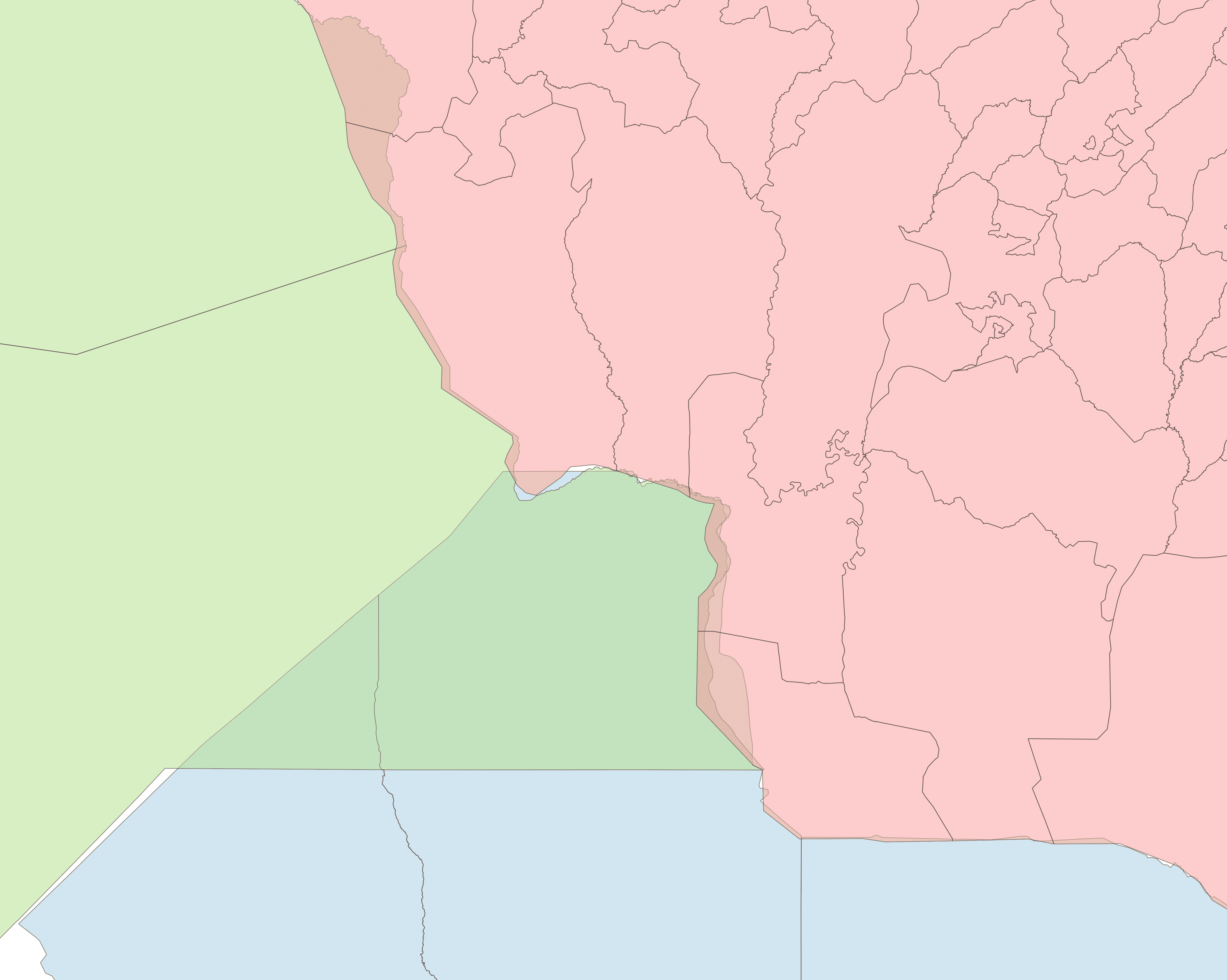
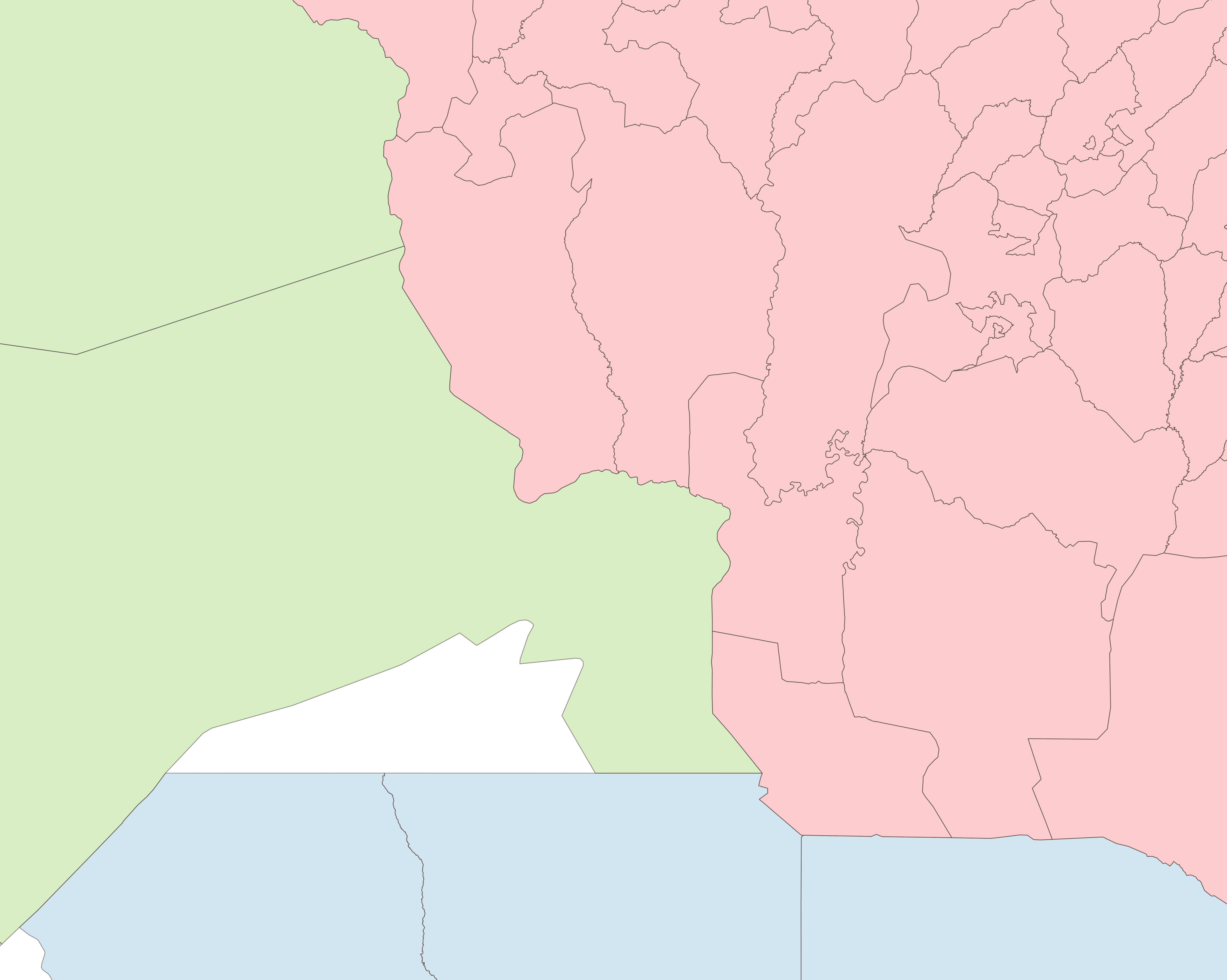
The other original use case envisioned for this tool is resolving edges between boundaries where there are significant gaps or overlaps. Where this occurs, a separate topologically clean layer is required to set boundary lines, after which the process is similar to the above.

Topologically clean ADM0 with areas of interest

Original boundaries	Clipped voronoi boundaries

Original boundaries (tri-point)	Clipped voronoi boundaries (tri-point)

Use Case 3: Improving coastlines¶

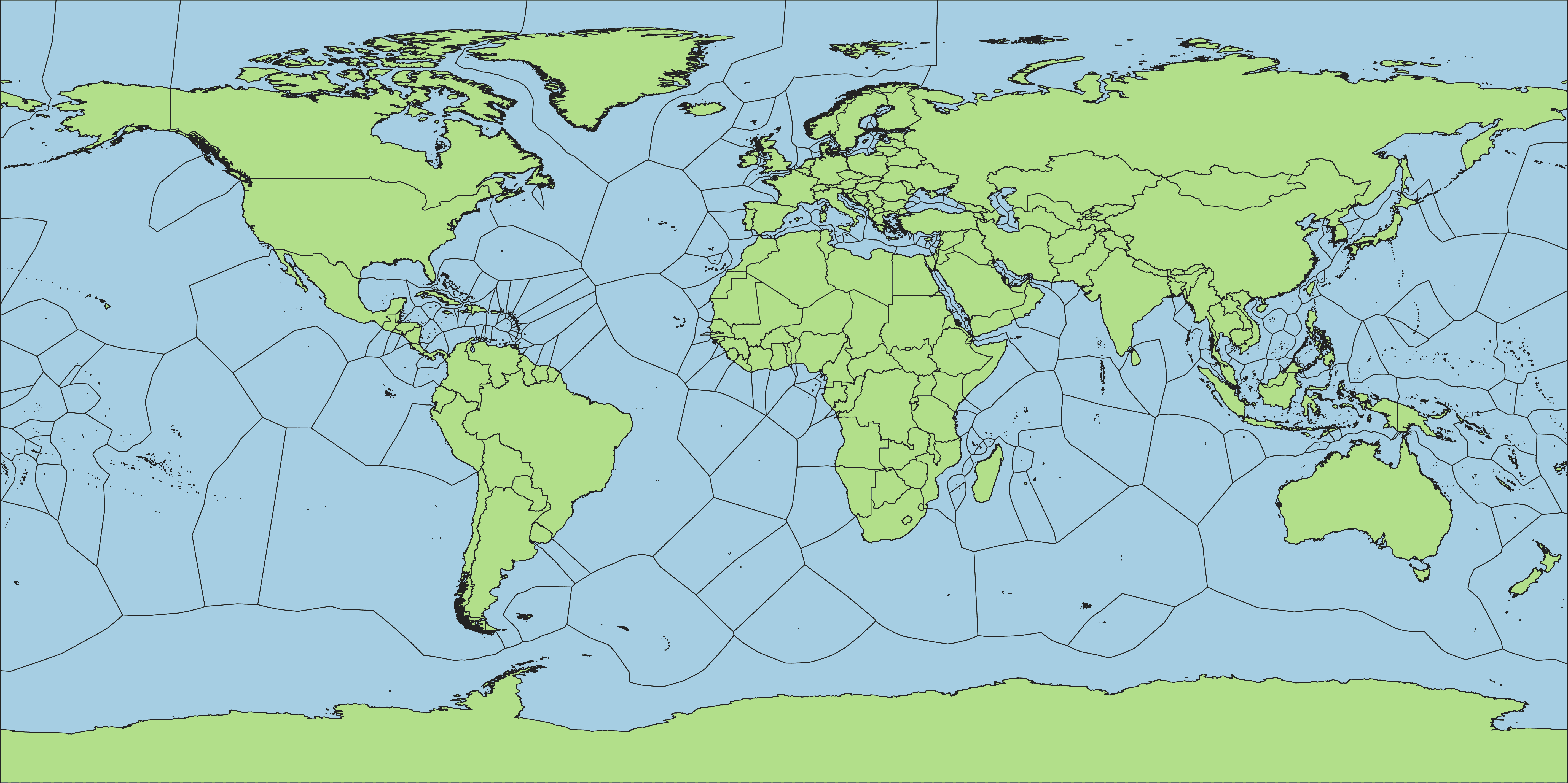
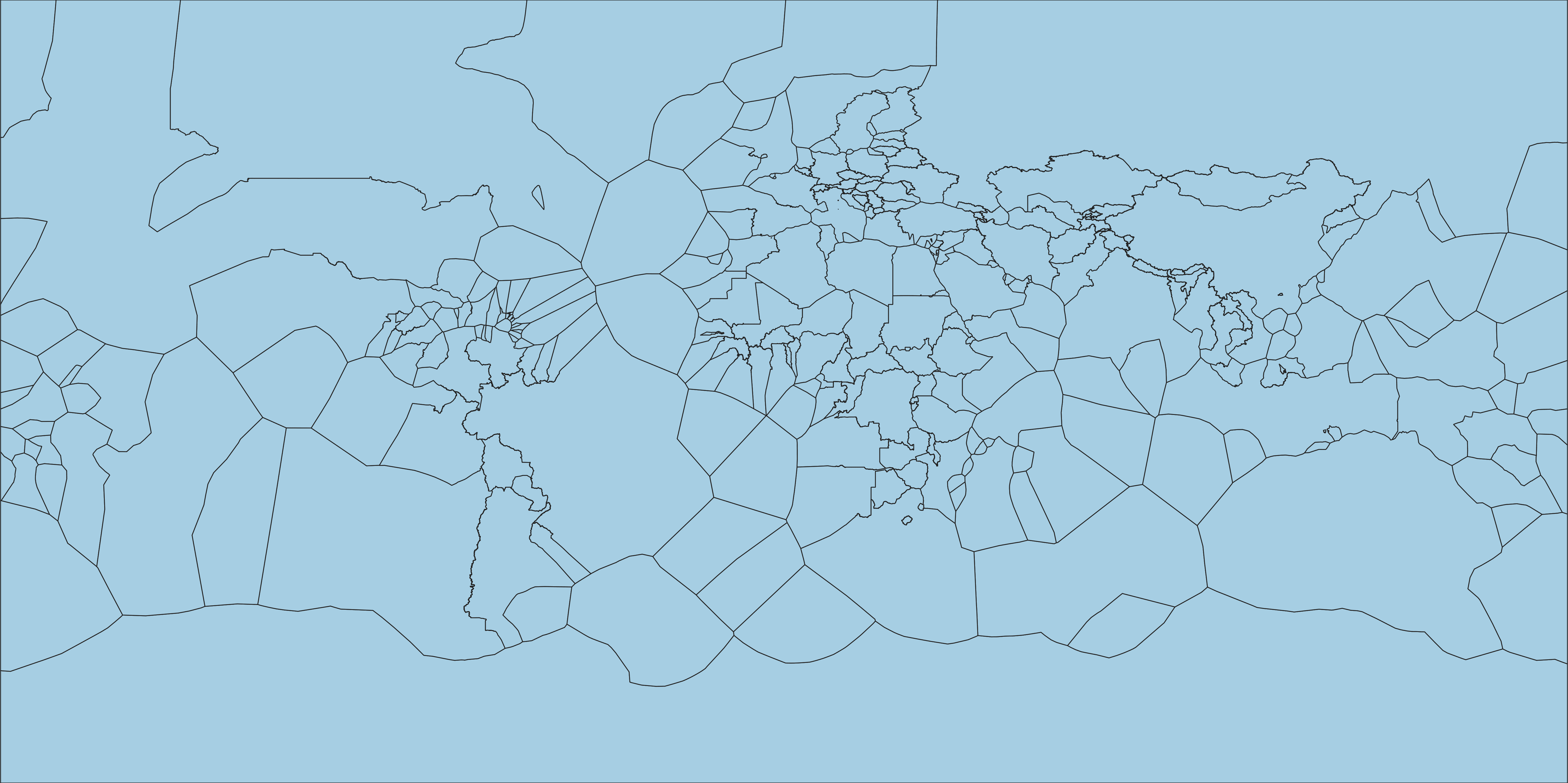
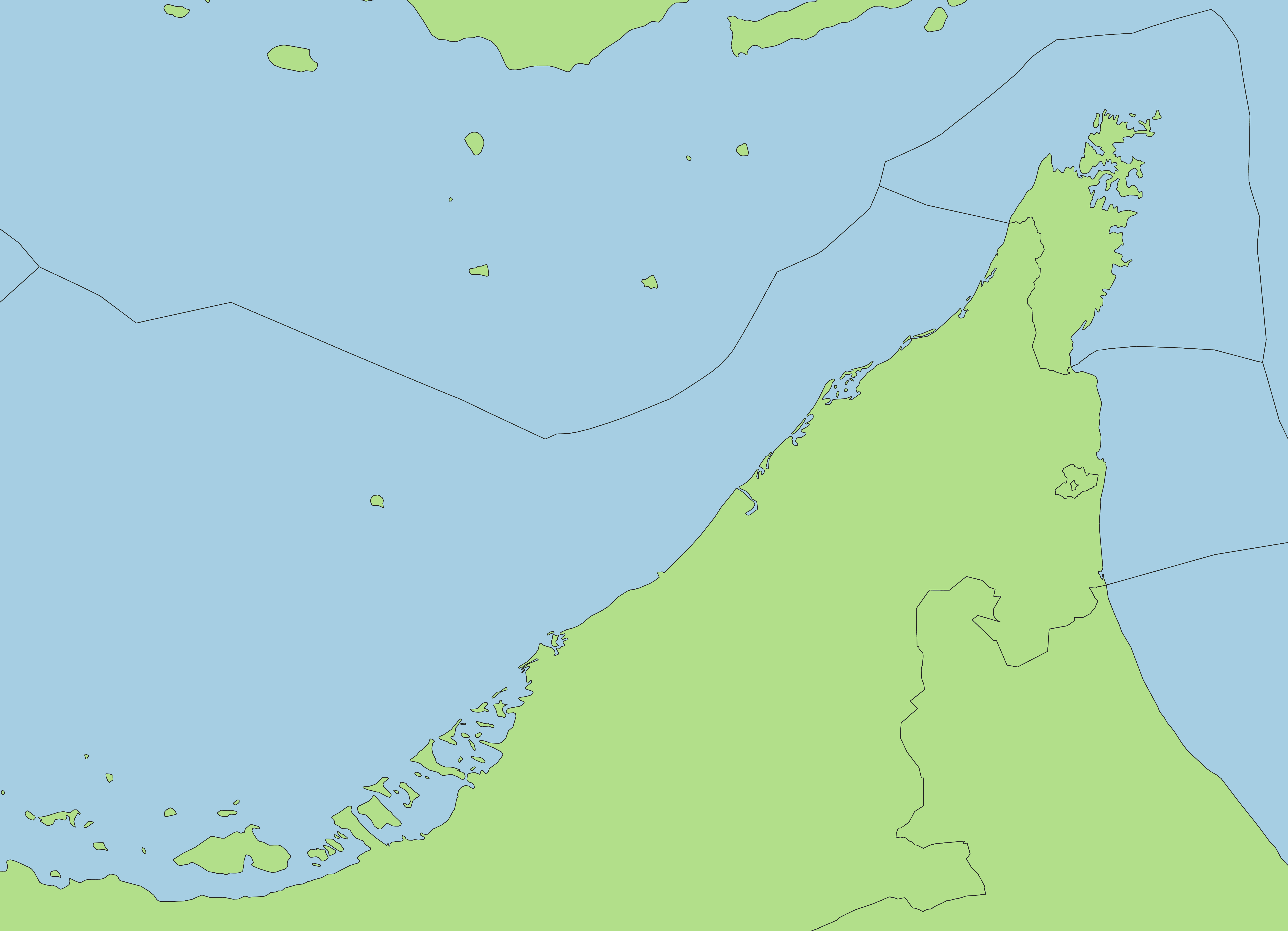
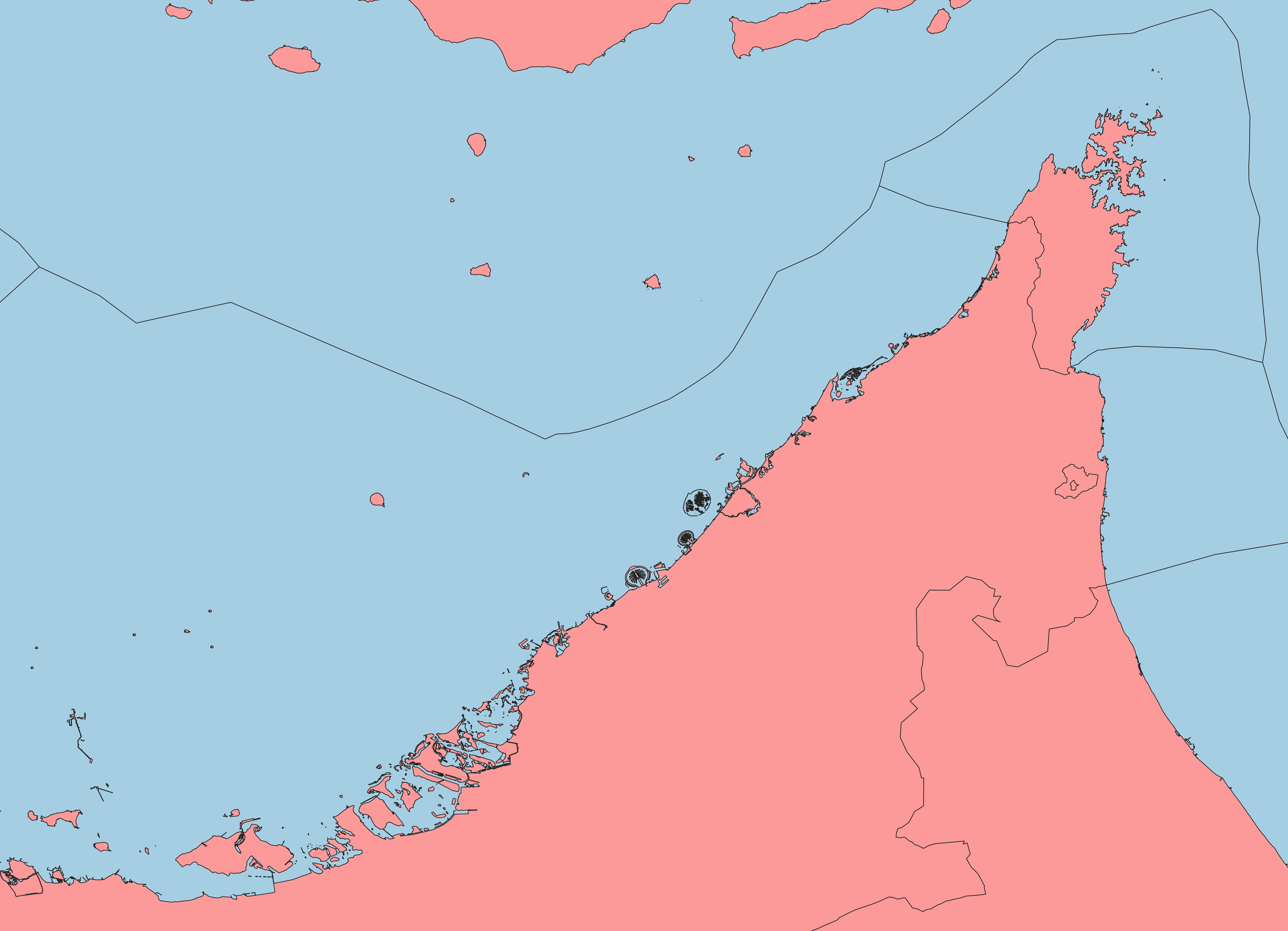
The use case above demonstrates how useful it is to have a topologically clean global ADM0 layer. Few portray disputed areas properly, and for those that do have accurate internal boundaries, coastlines may lack in detail compared to other sources. OpenStreetMap has very detailed coastline data available as Shapefiles, and this can be integrated with ADM0 datasets in the same way as above.

World ADM0 with Voronoi	Voronoi Only

Original ADM0	Coastline replaced with OSM