1  USA tracks radius model fit

Fitting model for wind radii to USA tracks

%load_ext jupyter_black
%load_ext autoreload
%autoreload 2

import ocha_lens as lens
import ocha_stratus as stratus
import pandas as pd
import numpy as np
import statsmodels.api as sm

from src.constants import *
from src.blob import PROJECT_PREFIX
from src.datasources.ibtracs import expand_quad_col

1.1 Processing data

Just extracting USA values from IBTrACS - can all be skipped if file is already saved to blob

# ds = lens.ibtracs.load_ibtracs(dataset="SP")

# df_storm = lens.ibtracs.get_storms(ds)

# gdf_tracks = lens.ibtracs.get_tracks(ds)

# speeds = [34, 50, 64]

quad_cols = [f"usa_r{x}" for x in speeds]

other_cols = ["sid", "usa_lat", "usa_lon", "usa_wind"]

var_cols = other_cols + quad_cols

ds_subset = ds[var_cols]
df_select = ds_subset.to_dataframe().reset_index()

df_ = lens.ibtracs.normalize_radii(df_select, radii_cols=quad_cols)
df_["valid_time"] = df_["time"].dt.round("min")
df_ = lens.ibtracs._convert_string_columns(df_, ["sid"])

df_ = df_[var_cols + ["valid_time"]]
df_ = df_[df_.valid_time.notna()]

df_

	sid	usa_lat	usa_lon	usa_wind	usa_r34	usa_r50	usa_r64	valid_time
0	1897005S10135	NaN	NaN	NaN	[nan, nan, nan, nan]	[nan, nan, nan, nan]	[nan, nan, nan, nan]	1897-01-04 12:00:00
1	1897005S10135	NaN	NaN	NaN	[nan, nan, nan, nan]	[nan, nan, nan, nan]	[nan, nan, nan, nan]	1897-01-04 15:00:00
2	1897005S10135	NaN	NaN	NaN	[nan, nan, nan, nan]	[nan, nan, nan, nan]	[nan, nan, nan, nan]	1897-01-04 18:00:00
3	1897005S10135	NaN	NaN	NaN	[nan, nan, nan, nan]	[nan, nan, nan, nan]	[nan, nan, nan, nan]	1897-01-04 21:00:00
4	1897005S10135	NaN	NaN	NaN	[nan, nan, nan, nan]	[nan, nan, nan, nan]	[nan, nan, nan, nan]	1897-01-05 00:00:00
...	...	...	...	...	...	...	...	...
447504	2025129S08138	-9.0	137.800003	35.0	[nan, nan, nan, nan]	[nan, nan, nan, nan]	[nan, nan, nan, nan]	2025-05-12 00:00:00
447505	2025129S08138	-8.6	137.500000	32.0	[nan, nan, nan, nan]	[nan, nan, nan, nan]	[nan, nan, nan, nan]	2025-05-12 03:00:00
447506	2025129S08138	-8.1	137.199997	29.0	[nan, nan, nan, nan]	[nan, nan, nan, nan]	[nan, nan, nan, nan]	2025-05-12 06:00:00
447507	2025129S08138	-7.9	137.000000	27.0	[nan, nan, nan, nan]	[nan, nan, nan, nan]	[nan, nan, nan, nan]	2025-05-12 09:00:00
447508	2025129S08138	-7.9	137.000000	25.0	[nan, nan, nan, nan]	[nan, nan, nan, nan]	[nan, nan, nan, nan]	2025-05-12 12:00:00

76381 rows × 8 columns

df_usa = df_.copy()

blob_name = f"{PROJECT_PREFIX}/processed/ibtracs/usa_only_wind_radii.parquet"

stratus.upload_parquet_to_blob(df_usa, blob_name)

1.2 Load and process data

df_usa = stratus.load_parquet_from_blob(blob_name)

query = """
SELECT *
FROM storms.ibtracs_storms
"""
with stratus.get_engine(stage="dev").connect() as conn:
    df_storms = pd.read_sql(query, conn)

df_usa = df_usa.merge(df_storms)

buffer_speeds = [34, 50, 64]
for buffer_speed in buffer_speeds:
    df_usa = expand_quad_col(df_usa, f"usa_r{buffer_speed}")

quads = ["ne", "nw", "se", "sw"]

Let’s see which quadrant tends to be the highest, and check where we have historical values for it.

df_usa[[f"usa_r34_{x}" for x in quads]].mean()

usa_r34_ne     96.604865
usa_r34_nw    100.630890
usa_r34_se     91.911209
usa_r34_sw     86.478483
dtype: float64

df_usa.groupby("season")["usa_r34_nw"].count().plot()

df_usa[df_usa["season"] >= 1980].groupby("season")["usa_r34_nw"].count()

season
1980      0
1981      0
1982      0
1983      0
1984      0
1985      0
1986      0
1987      0
1988      0
1989      0
1990      0
1991      0
1992      0
1993      0
1994      0
1995      0
1996      0
1997      0
1998      0
1999      0
2000      0
2001      0
2002     62
2003    244
2004    206
2005    342
2006    240
2007    201
2008    189
2009    124
2010    377
2011    288
2012    123
2013    267
2014    276
2015    317
2016    404
2017    228
2018    304
2019    351
2020    316
2021    232
2022    189
2023    185
2024    235
2025    179
Name: usa_r34_nw, dtype: int64

Looks like JTWC started fully recording this in the 2003 season, so we can filter from only then onwards.

min_season = 2003

df_usa_recent = df_usa[df_usa["season"] >= min_season]
df_usa_recent = df_usa_recent.dropna(subset="usa_wind")

radius_cols = [
    f"usa_r{speed}_{quad}" for speed in buffer_speeds for quad in quads
]

Since we now know that we’re only including years where (presumably) JTWC would record the wind radius if it exists, we can assume that if it’s missing, it should be zero.

df_usa_recent[radius_cols] = df_usa_recent[radius_cols].fillna(0)

We can calculate the mean radius. We won’t bother with trying to model the individual quadrants just for simplicity.

for speed in buffer_speeds:
    cols = [f"usa_r{speed}_{quad}" for quad in quads]
    df_usa_recent[f"usa_r{speed}_mean"] = df_usa_recent[cols].mean(axis=1)

df_usa_recent

	sid	usa_lat	usa_lon	usa_wind	usa_r34	usa_r50	usa_r64	valid_time	atcf_id	number	...	usa_r64_mean_log	usa_lat_log	usa_r34_mean_pred	usa_r50_mean_pred	usa_r64_mean_pred	usa_lat_abs	usa_lat_abs_log	usa_r34_mean_log_pred	usa_r50_mean_log_pred	usa_r64_mean_log_pred
61342	2002335S13182	-13.2	-178.300003	25.0	[nan, nan, nan, nan]	[nan, nan, nan, nan]	[nan, nan, nan, nan]	2002-12-01 06:00:00	SH042003	94	...	-inf	NaN	0.000000	0.0	0.0	13.2	2.580217	3.738919	2.634926	2.234446
61343	2002335S13182	-13.4	-178.199997	25.0	[nan, nan, nan, nan]	[nan, nan, nan, nan]	[nan, nan, nan, nan]	2002-12-01 09:00:00	SH042003	94	...	-inf	NaN	0.000000	0.0	0.0	13.4	2.595255	3.747939	2.646504	2.242664
61344	2002335S13182	-13.5	-178.000000	25.0	[nan, nan, nan, nan]	[nan, nan, nan, nan]	[nan, nan, nan, nan]	2002-12-01 12:00:00	SH042003	94	...	-inf	NaN	0.000000	0.0	0.0	13.5	2.602690	3.752399	2.652228	2.246726
61345	2002335S13182	-13.7	-177.800003	25.0	[nan, nan, nan, nan]	[nan, nan, nan, nan]	[nan, nan, nan, nan]	2002-12-01 15:00:00	SH042003	94	...	-inf	NaN	0.000000	0.0	0.0	13.7	2.617396	3.761221	2.663549	2.254763
61346	2002335S13182	-13.8	-177.600006	25.0	[nan, nan, nan, nan]	[nan, nan, nan, nan]	[nan, nan, nan, nan]	2002-12-01 18:00:00	SH042003	94	...	-inf	NaN	0.000000	0.0	0.0	13.8	2.624669	3.765584	2.669149	2.258737
...	...	...	...	...	...	...	...	...	...	...	...	...	...	...	...	...	...	...	...	...	...
76376	2025129S08138	-9.0	137.800003	35.0	[nan, nan, nan, nan]	[nan, nan, nan, nan]	[nan, nan, nan, nan]	2025-05-12 00:00:00	SH322025	27	...	-inf	NaN	40.729703	0.0	0.0	9.0	2.197225	3.706958	2.609259	2.256789
76377	2025129S08138	-8.6	137.500000	32.0	[nan, nan, nan, nan]	[nan, nan, nan, nan]	[nan, nan, nan, nan]	2025-05-12 03:00:00	SH322025	27	...	-inf	NaN	0.000000	0.0	0.0	8.6	2.151762	3.627011	2.502567	2.170257
76378	2025129S08138	-8.1	137.199997	29.0	[nan, nan, nan, nan]	[nan, nan, nan, nan]	[nan, nan, nan, nan]	2025-05-12 06:00:00	SH322025	27	...	-inf	NaN	0.000000	0.0	0.0	8.1	2.091864	3.533216	2.377698	2.069760
76379	2025129S08138	-7.9	137.000000	27.0	[nan, nan, nan, nan]	[nan, nan, nan, nan]	[nan, nan, nan, nan]	2025-05-12 09:00:00	SH322025	27	...	-inf	NaN	0.000000	0.0	0.0	7.9	2.066863	3.476214	2.301281	2.006906
76380	2025129S08138	-7.9	137.000000	25.0	[nan, nan, nan, nan]	[nan, nan, nan, nan]	[nan, nan, nan, nan]	2025-05-12 12:00:00	SH322025	27	...	-inf	NaN	0.000000	0.0	0.0	7.9	2.066863	3.430975	2.239710	1.953926

10955 rows × 43 columns

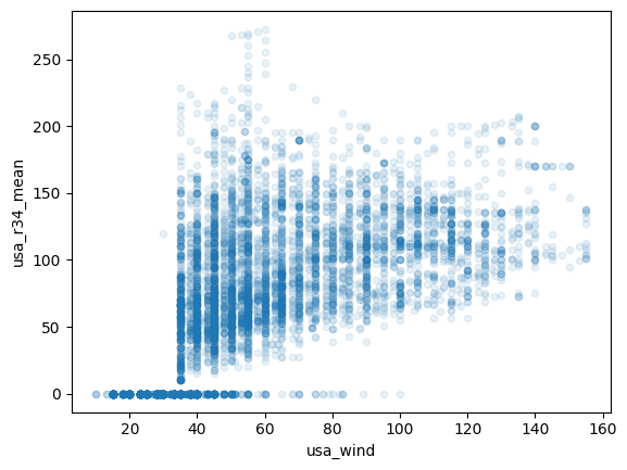
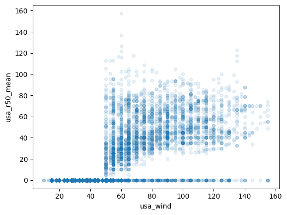
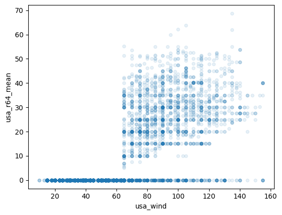
Let’s see how things look for each buffer speed.

for speed in buffer_speeds:
    df_usa_recent.plot.scatter(
        x="usa_wind",
        y=f"usa_r{speed}_mean",
        alpha=0.1,
    )

It’s interesting, it looks like for many points there is no buffer defined despite the wind speed being high enough. We can filter these out when fitting the regression.

1.3 Regression

1.3.1 Compare various methods

Here we can compare: - Linear vs. log-log (log in the results table) - Whether we should also include latitude (or only wind speed) (dof in the results table)

First we set up the columns.

mean_quad_cols = [f"usa_r{speed}_mean" for speed in buffer_speeds]

df_usa_recent["usa_lat_abs"] = df_usa_recent["usa_lat"].abs()

for col in ["usa_wind", "usa_lat_abs"] + mean_quad_cols:
    df_usa_recent[f"{col}_log"] = np.log(df_usa_recent[col])

Then we iterate over the possible setups.

dicts = []
for col in mean_quad_cols:
    print(col)
    for log_str in ["", "_log"]:
        target_col = f"{col}{log_str}"
        for var_cols in [
            [f"usa_wind{log_str}"],
            [f"usa_wind{log_str}", f"usa_lat_abs{log_str}"],
        ]:
            df_reg = df_usa_recent[[target_col] + var_cols].dropna()
            # exclude zero values (which would show up as -np.inf for the log)
            df_reg = df_reg[df_reg[target_col] > 0]
            X = df_reg[var_cols]
            y = df_reg[target_col]
            X = sm.add_constant(X)
            model = sm.OLS(y, X).fit()
            print(var_cols)
            display(model.summary())
            dicts.append(
                {
                    "col": col,
                    "dof": len(var_cols),
                    "log": log_str,
                    "r2adj": model.rsquared_adj,
                }
            )

usa_r34_mean
['usa_wind']

OLS Regression Results

Dep. Variable:	usa_r34_mean	R-squared:	0.143
Model:	OLS	Adj. R-squared:	0.143
Method:	Least Squares	F-statistic:	972.1
Date:	Tue, 30 Sep 2025	Prob (F-statistic):	1.79e-197
Time:	13:53:31	Log-Likelihood:	-29327.
No. Observations:	5817	AIC:	5.866e+04
Df Residuals:	5815	BIC:	5.867e+04
Df Model:	1
Covariance Type:	nonrobust

	coef	std err	t	P>|t|	[0.025	0.975]
const	56.2839	1.300	43.282	0.000	53.735	58.833
usa_wind	0.5662	0.018	31.178	0.000	0.531	0.602

Omnibus:	824.492	Durbin-Watson:	0.121
Prob(Omnibus):	0.000	Jarque-Bera (JB):	1312.977
Skew:	0.980	Prob(JB):	7.77e-286
Kurtosis:	4.255	Cond. No.	190.

Notes:
[1] Standard Errors assume that the covariance matrix of the errors is correctly specified.

['usa_wind', 'usa_lat_abs']

OLS Regression Results

Dep. Variable:	usa_r34_mean	R-squared:	0.317
Model:	OLS	Adj. R-squared:	0.317
Method:	Least Squares	F-statistic:	1348.
Date:	Tue, 30 Sep 2025	Prob (F-statistic):	0.00
Time:	13:53:32	Log-Likelihood:	-28669.
No. Observations:	5817	AIC:	5.734e+04
Df Residuals:	5814	BIC:	5.736e+04
Df Model:	2
Covariance Type:	nonrobust

	coef	std err	t	P>|t|	[0.025	0.975]
const	-8.6823	2.051	-4.233	0.000	-12.703	-4.662
usa_wind	0.6521	0.016	39.831	0.000	0.620	0.684
usa_lat_abs	3.2433	0.084	38.429	0.000	3.078	3.409

Omnibus:	403.791	Durbin-Watson:	0.117
Prob(Omnibus):	0.000	Jarque-Bera (JB):	523.749
Skew:	0.631	Prob(JB):	1.86e-114
Kurtosis:	3.755	Cond. No.	344.

Notes:
[1] Standard Errors assume that the covariance matrix of the errors is correctly specified.

['usa_wind_log']

OLS Regression Results

Dep. Variable:	usa_r34_mean_log	R-squared:	0.189
Model:	OLS	Adj. R-squared:	0.189
Method:	Least Squares	F-statistic:	1358.
Date:	Tue, 30 Sep 2025	Prob (F-statistic):	2.44e-267
Time:	13:53:32	Log-Likelihood:	-3329.5
No. Observations:	5817	AIC:	6663.
Df Residuals:	5815	BIC:	6676.
Df Model:	1
Covariance Type:	nonrobust

	coef	std err	t	P>|t|	[0.025	0.975]
const	2.1968	0.061	35.946	0.000	2.077	2.317
usa_wind_log	0.5444	0.015	36.849	0.000	0.515	0.573

Omnibus:	219.114	Durbin-Watson:	0.188
Prob(Omnibus):	0.000	Jarque-Bera (JB):	373.137
Skew:	-0.321	Prob(JB):	9.42e-82
Kurtosis:	4.062	Cond. No.	47.6

Notes:
[1] Standard Errors assume that the covariance matrix of the errors is correctly specified.

['usa_wind_log', 'usa_lat_abs_log']

OLS Regression Results

Dep. Variable:	usa_r34_mean_log	R-squared:	0.315
Model:	OLS	Adj. R-squared:	0.315
Method:	Least Squares	F-statistic:	1337.
Date:	Tue, 30 Sep 2025	Prob (F-statistic):	0.00
Time:	13:53:32	Log-Likelihood:	-2839.2
No. Observations:	5817	AIC:	5684.
Df Residuals:	5814	BIC:	5704.
Df Model:	2
Covariance Type:	nonrobust

	coef	std err	t	P>|t|	[0.025	0.975]
const	0.2990	0.081	3.701	0.000	0.141	0.457
usa_wind_log	0.5878	0.014	43.076	0.000	0.561	0.615
usa_lat_abs_log	0.5999	0.018	32.672	0.000	0.564	0.636

Omnibus:	426.097	Durbin-Watson:	0.186
Prob(Omnibus):	0.000	Jarque-Bera (JB):	777.888
Skew:	-0.529	Prob(JB):	1.21e-169
Kurtosis:	4.446	Cond. No.	81.9

Notes:
[1] Standard Errors assume that the covariance matrix of the errors is correctly specified.

usa_r50_mean
['usa_wind']

OLS Regression Results

Dep. Variable:	usa_r50_mean	R-squared:	0.110
Model:	OLS	Adj. R-squared:	0.110
Method:	Least Squares	F-statistic:	364.3
Date:	Tue, 30 Sep 2025	Prob (F-statistic):	1.13e-76
Time:	13:53:32	Log-Likelihood:	-12906.
No. Observations:	2953	AIC:	2.582e+04
Df Residuals:	2951	BIC:	2.583e+04
Df Model:	1
Covariance Type:	nonrobust

	coef	std err	t	P>|t|	[0.025	0.975]
const	25.1539	1.245	20.207	0.000	22.713	27.595
usa_wind	0.2776	0.015	19.087	0.000	0.249	0.306

Omnibus:	324.252	Durbin-Watson:	0.163
Prob(Omnibus):	0.000	Jarque-Bera (JB):	454.674
Skew:	0.851	Prob(JB):	1.86e-99
Kurtosis:	3.893	Cond. No.	302.

Notes:
[1] Standard Errors assume that the covariance matrix of the errors is correctly specified.

['usa_wind', 'usa_lat_abs']

OLS Regression Results

Dep. Variable:	usa_r50_mean	R-squared:	0.308
Model:	OLS	Adj. R-squared:	0.308
Method:	Least Squares	F-statistic:	657.0
Date:	Tue, 30 Sep 2025	Prob (F-statistic):	9.99e-237
Time:	13:53:32	Log-Likelihood:	-12534.
No. Observations:	2953	AIC:	2.507e+04
Df Residuals:	2950	BIC:	2.509e+04
Df Model:	2
Covariance Type:	nonrobust

	coef	std err	t	P>|t|	[0.025	0.975]
const	-15.6852	1.783	-8.799	0.000	-19.180	-12.190
usa_wind	0.3417	0.013	26.261	0.000	0.316	0.367
usa_lat_abs	1.9760	0.068	29.077	0.000	1.843	2.109

Omnibus:	130.622	Durbin-Watson:	0.169
Prob(Omnibus):	0.000	Jarque-Bera (JB):	161.339
Skew:	0.470	Prob(JB):	9.24e-36
Kurtosis:	3.655	Cond. No.	501.

Notes:
[1] Standard Errors assume that the covariance matrix of the errors is correctly specified.

['usa_wind_log']

OLS Regression Results

Dep. Variable:	usa_r50_mean_log	R-squared:	0.172
Model:	OLS	Adj. R-squared:	0.171
Method:	Least Squares	F-statistic:	612.0
Date:	Tue, 30 Sep 2025	Prob (F-statistic):	6.06e-123
Time:	13:53:32	Log-Likelihood:	-1763.5
No. Observations:	2953	AIC:	3531.
Df Residuals:	2951	BIC:	3543.
Df Model:	1
Covariance Type:	nonrobust

	coef	std err	t	P>|t|	[0.025	0.975]
const	0.7087	0.124	5.720	0.000	0.466	0.952
usa_wind_log	0.7005	0.028	24.739	0.000	0.645	0.756

Omnibus:	120.386	Durbin-Watson:	0.299
Prob(Omnibus):	0.000	Jarque-Bera (JB):	201.049
Skew:	-0.344	Prob(JB):	2.20e-44
Kurtosis:	4.078	Cond. No.	70.5

Notes:
[1] Standard Errors assume that the covariance matrix of the errors is correctly specified.

['usa_wind_log', 'usa_lat_abs_log']

OLS Regression Results

Dep. Variable:	usa_r50_mean_log	R-squared:	0.329
Model:	OLS	Adj. R-squared:	0.328
Method:	Least Squares	F-statistic:	721.7
Date:	Tue, 30 Sep 2025	Prob (F-statistic):	7.12e-256
Time:	13:53:32	Log-Likelihood:	-1453.6
No. Observations:	2953	AIC:	2913.
Df Residuals:	2950	BIC:	2931.
Df Model:	2
Covariance Type:	nonrobust

	coef	std err	t	P>|t|	[0.025	0.975]
const	-1.9267	0.150	-12.835	0.000	-2.221	-1.632
usa_wind_log	0.8000	0.026	31.032	0.000	0.749	0.851
usa_lat_abs_log	0.7699	0.029	26.245	0.000	0.712	0.827

Omnibus:	316.881	Durbin-Watson:	0.312
Prob(Omnibus):	0.000	Jarque-Bera (JB):	629.490
Skew:	-0.687	Prob(JB):	2.03e-137
Kurtosis:	4.797	Cond. No.	112.

Notes:
[1] Standard Errors assume that the covariance matrix of the errors is correctly specified.

usa_r64_mean
['usa_wind']

OLS Regression Results

Dep. Variable:	usa_r64_mean	R-squared:	0.078
Model:	OLS	Adj. R-squared:	0.077
Method:	Least Squares	F-statistic:	152.3
Date:	Tue, 30 Sep 2025	Prob (F-statistic):	1.16e-33
Time:	13:53:32	Log-Likelihood:	-6758.1
No. Observations:	1814	AIC:	1.352e+04
Df Residuals:	1812	BIC:	1.353e+04
Df Model:	1
Covariance Type:	nonrobust

	coef	std err	t	P>|t|	[0.025	0.975]
const	15.3072	1.113	13.756	0.000	13.125	17.490
usa_wind	0.1404	0.011	12.342	0.000	0.118	0.163

Omnibus:	71.506	Durbin-Watson:	0.220
Prob(Omnibus):	0.000	Jarque-Bera (JB):	71.794
Skew:	0.452	Prob(JB):	2.57e-16
Kurtosis:	2.635	Cond. No.	462.

Notes:
[1] Standard Errors assume that the covariance matrix of the errors is correctly specified.

['usa_wind', 'usa_lat_abs']

OLS Regression Results

Dep. Variable:	usa_r64_mean	R-squared:	0.187
Model:	OLS	Adj. R-squared:	0.186
Method:	Least Squares	F-statistic:	208.2
Date:	Tue, 30 Sep 2025	Prob (F-statistic):	4.09e-82
Time:	13:53:32	Log-Likelihood:	-6643.6
No. Observations:	1814	AIC:	1.329e+04
Df Residuals:	1811	BIC:	1.331e+04
Df Model:	2
Covariance Type:	nonrobust

	coef	std err	t	P>|t|	[0.025	0.975]
const	-3.0654	1.574	-1.948	0.052	-6.152	0.021
usa_wind	0.1709	0.011	15.738	0.000	0.150	0.192
usa_lat_abs	0.8783	0.056	15.610	0.000	0.768	0.989

Omnibus:	35.723	Durbin-Watson:	0.224
Prob(Omnibus):	0.000	Jarque-Bera (JB):	32.986
Skew:	0.284	Prob(JB):	6.87e-08
Kurtosis:	2.663	Cond. No.	706.

Notes:
[1] Standard Errors assume that the covariance matrix of the errors is correctly specified.

['usa_wind_log']

OLS Regression Results

Dep. Variable:	usa_r64_mean_log	R-squared:	0.100
Model:	OLS	Adj. R-squared:	0.099
Method:	Least Squares	F-statistic:	201.2
Date:	Tue, 30 Sep 2025	Prob (F-statistic):	2.22e-43
Time:	13:53:32	Log-Likelihood:	-809.93
No. Observations:	1814	AIC:	1624.
Df Residuals:	1812	BIC:	1635.
Df Model:	1
Covariance Type:	nonrobust

	coef	std err	t	P>|t|	[0.025	0.975]
const	0.6100	0.189	3.231	0.001	0.240	0.980
usa_wind_log	0.5895	0.042	14.183	0.000	0.508	0.671

Omnibus:	41.865	Durbin-Watson:	0.328
Prob(Omnibus):	0.000	Jarque-Bera (JB):	44.192
Skew:	-0.376	Prob(JB):	2.53e-10
Kurtosis:	2.860	Cond. No.	101.

Notes:
[1] Standard Errors assume that the covariance matrix of the errors is correctly specified.

['usa_wind_log', 'usa_lat_abs_log']

OLS Regression Results

Dep. Variable:	usa_r64_mean_log	R-squared:	0.197
Model:	OLS	Adj. R-squared:	0.196
Method:	Least Squares	F-statistic:	221.8
Date:	Tue, 30 Sep 2025	Prob (F-statistic):	6.82e-87
Time:	13:53:32	Log-Likelihood:	-706.68
No. Observations:	1814	AIC:	1419.
Df Residuals:	1811	BIC:	1436.
Df Model:	2
Covariance Type:	nonrobust

	coef	std err	t	P>|t|	[0.025	0.975]
const	-1.3914	0.224	-6.212	0.000	-1.831	-0.952
usa_wind_log	0.6884	0.040	17.278	0.000	0.610	0.767
usa_lat_abs_log	0.5464	0.037	14.777	0.000	0.474	0.619

Omnibus:	74.527	Durbin-Watson:	0.333
Prob(Omnibus):	0.000	Jarque-Bera (JB):	83.100
Skew:	-0.523	Prob(JB):	9.02e-19
Kurtosis:	3.066	Cond. No.	148.

Notes:
[1] Standard Errors assume that the covariance matrix of the errors is correctly specified.

df_results = pd.DataFrame(dicts)

df_results

	col	dof	log	r2adj
0	usa_r34_mean	1		0.143076
1	usa_r34_mean	2		0.316536
2	usa_r34_mean	1	_log	0.189163
3	usa_r34_mean	2	_log	0.314823
4	usa_r50_mean	1		0.109584
5	usa_r50_mean	2		0.307701
6	usa_r50_mean	1	_log	0.171486
7	usa_r50_mean	2	_log	0.328087
8	usa_r64_mean	1		0.077041
9	usa_r64_mean	2		0.186051
10	usa_r64_mean	1	_log	0.099429
11	usa_r64_mean	2	_log	0.195881

From the results (column r2adj is the adjusted \(R^2\) value) above it looks like: 1. Log-log performs better than linear 2. Including latitude (dof=2) is better than only wind So, we’ll go with that.

1.3.2 Make predictions

dicts_params = []
for col in mean_quad_cols:
    df_reg = df_usa_recent[
        ["sid", "valid_time", "usa_wind_log", "usa_lat_abs_log", f"{col}_log"]
    ].dropna()
    df_reg = df_reg[df_reg[f"{col}_log"] > 0]
    X = df_reg[["usa_wind_log", "usa_lat_abs_log"]]
    y = df_reg[f"{col}_log"]
    X = sm.add_constant(X)
    model = sm.OLS(y, X).fit()
    dicts_params.append({"col": col, "params": model.params})
    X_pred = df_usa_recent[["usa_wind_log", "usa_lat_abs_log"]]
    X_pred = sm.add_constant(X_pred)
    df_usa_recent[f"{col}_log_pred"] = model.predict(X_pred)

Here are the parameters which we will save in src.constants so we can apply them to new forecasts:

dicts_params

[{'col': 'usa_r34_mean',
  'params': const              0.299034
  usa_wind_log       0.587814
  usa_lat_abs_log    0.599866
  dtype: float64},
 {'col': 'usa_r50_mean',
  'params': const             -1.926702
  usa_wind_log       0.800029
  usa_lat_abs_log    0.769871
  dtype: float64},
 {'col': 'usa_r64_mean',
  'params': const             -1.391375
  usa_wind_log       0.688399
  usa_lat_abs_log    0.546447
  dtype: float64}]

We also just want to set anywhere with a maximum wind speed lower than the buffer speed to a radius of 0.

log_pred_cols = [f"usa_r{speed}_mean_log_pred" for speed in buffer_speeds]

for speed in buffer_speeds:
    df_usa_recent[f"usa_r{speed}_mean_pred"] = np.exp(
        df_usa_recent[f"usa_r{speed}_mean_log_pred"]
    )
    df_usa_recent[f"usa_r{speed}_mean_pred"] = df_usa_recent.apply(
        lambda row: 0
        if row["usa_wind"] < speed
        else row[f"usa_r{speed}_mean_pred"],
        axis=1,
    )

1.3.3 Plot results

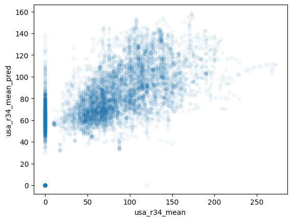
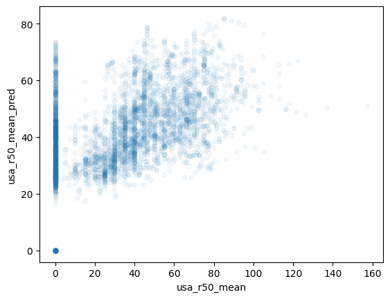
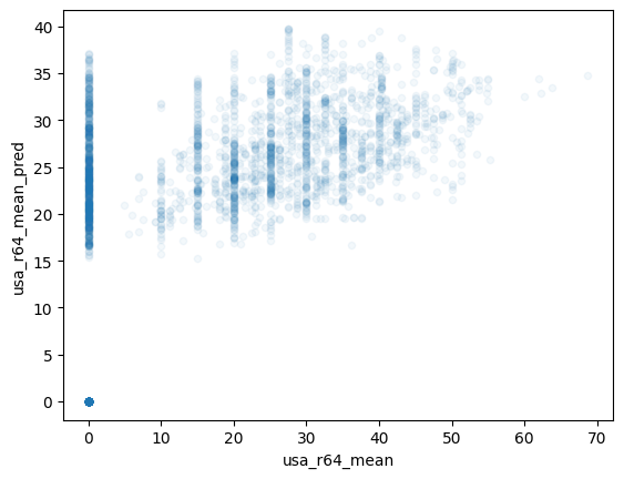
Here we plot the results - looks ok, although we often predict a non-zero radius when the radius. But this could be from the weird points above where it’s possible that JTWC didn’t calculate a radius.

for col in mean_quad_cols:
    df_usa_recent.plot.scatter(
        x=f"{col}",
        y=f"{col}_pred",
        alpha=0.05,
    )

We can also calculate the \(R^2\) and correlation (including the zeros, so pessimistic estimate).

def calc_r2(y_pred, y_true, k):
    n = len(y_true)
    ss_res = np.sum((y_true - y_pred) ** 2)
    ss_tot = np.sum((y_true - np.mean(y_true)) ** 2)
    r2 = 1 - ss_res / ss_tot
    r2_adj = 1 - (1 - r2) * (n - 1) / (n - k - 1)
    return r2, r2_adj

for speed in buffer_speeds:
    print(speed)
    print("corr:")
    print(
        df_usa_recent[[f"usa_r{speed}_mean", f"usa_r{speed}_mean_pred"]]
        .corr()
        .iloc[0, 1]
    )
    print("r2, r2adj:")
    r2, r2_adj = calc_r2(
        df_usa_recent[f"usa_r{speed}_mean_pred"],
        df_usa_recent[f"usa_r{speed}_mean"],
        2,
    )
    print(r2, r2_adj)
    print()

34
corr:
0.81989964048842
r2, r2adj:
0.6703863098074991 0.6703261173878146

50
corr:
0.7860493517451125
r2, r2adj:
0.5824097176915151 0.5823334594222842

64
corr:
0.7976896352206827
r2, r2adj:
0.589050204675589 0.588975159059204

1.3.4 Plot examples

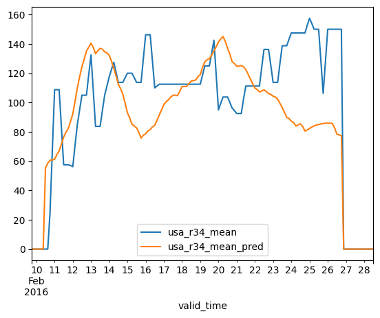
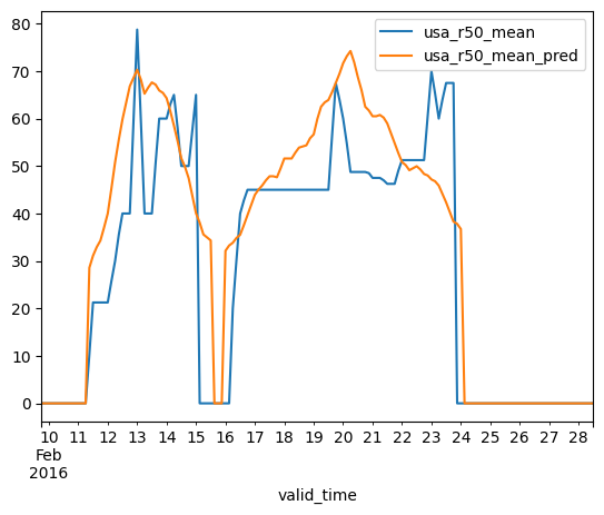
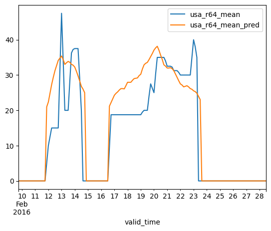
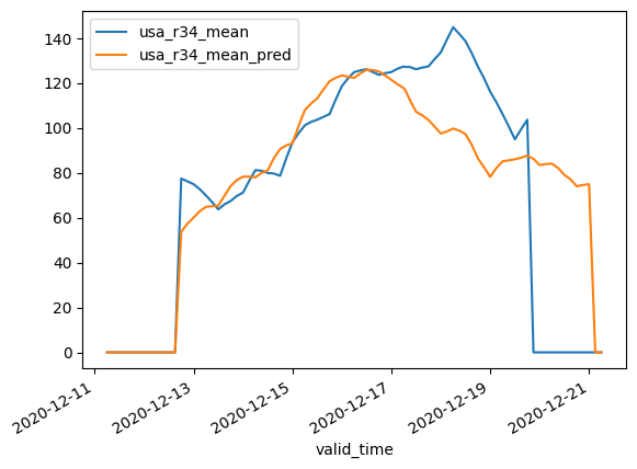
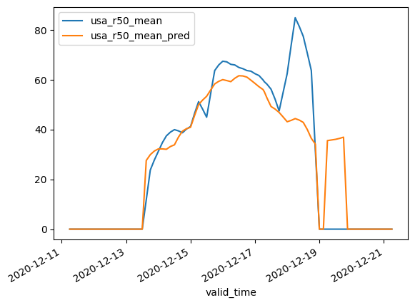
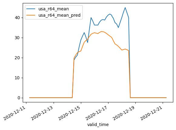
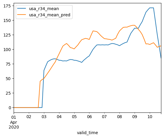
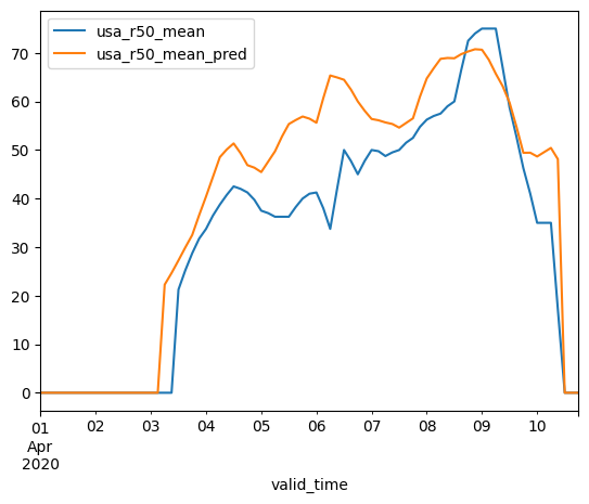
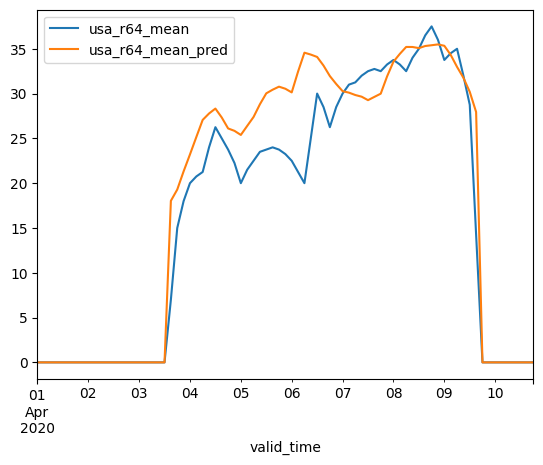
Plot examples for Winston, Yasa, and Harold. Looks not bad.

for sid in [WINSTON_SID, YASA_SID, HAROLD_SID]:
    for speed in buffer_speeds:
        df_usa_recent.set_index("sid").loc[sid].plot(
            x="valid_time", y=[f"usa_r{speed}_mean", f"usa_r{speed}_mean_pred"]
        )